This may be the night that my dreams might let me know
All the stars are closer

— “All the Stars” by Kendrick Lamar, SZA

Where shall we begin our mathematical conversation? Let’s head back to Kindergarten and develop number systems from the ground up.

1.1 Foundations

Arithmetic

Hold out your hands, palms up, fists closed, and count with me.

\(0\) (no fingers to start), \(1\) (left thumb), \(2\) (left index finger), \(3\) (left middle finger), and so on. The numbers we learn to count on our fingers and toes are commonly known as the natural numbers.

\(\mathbb{N}\) is the set of natural numbers: \(\{0, 1, 2, 3, ...\}\)

A set is a group of unique objects. We could easily talk about sets of numbers, or members of the hip hop duo OutKast, or the Harry Potter novels… any group will do. My question is this: what can we actually do with the set?

Hopefully you experienced the joy of playing with blocks at some point. Whether Multilink or the video game Minecraft, it’s natural to put blocks together and take them apart again. This sort of play is where we’ll start our discussion of arithmetic.

You can visualize any mathematical idea. For starters, imagine that I gave you a stack of \(2\) blocks and another stack of \(3\) blocks. What would happen if you snapped them together?

Figure 1.1 Block addition

Snapping blocks together is one way to think about addition. It has a nice intuitive feel. Plus you can go try it out if you have some LEGOs lying around.

As with many ideas we’ll encounter together, there’s more than one way to view addition.

Figure 1.2 Another way to add

It turns out that you can add blocks together in either order and still get the same result. Mathematicians call this the commutative property of addition.

Now what happens when you break blocks apart?

Figure 1.3 Block subtraction

OK, we can put blocks together and take some blocks away, but does that really have anything to do with math?

Let’s try multiplication. The mathematical expression \(3 \times 2\) just means “put \(3\) copies of the number \(2\) together.”

Figure 1.4 Block multiplication

Similar to addtion, \(3 \times 2\) also means “put \(2\) copies of the number \(3\) together.”

Figure 1.5 Multiplication is also commutative

How about division? The expression \(6 \div 3\) means “subtract \(3\) from \(6\) repeatedly until you reach a number smaller than \(3\).” The result, or value, produced by division is the number of times you subtract successfully.

OK, let’s give it a go.

Figure 1.6 Block division

You can also think of division as an instruction to break a stack of blocks into sub-stacks of equal size. In this view, \(6 \div 3\) means “break \(6\) into \(3\) identical pieces.” The value produced is the size of identical sub-stacks.

And any leftover blocks? We’ll get to those in a bit.

Figure 1.7 Block division as sub-stacks

Thinking of division this way, it’s difficult to imagine breaking something into \(0\) pieces. In fact, the idea is so troublesome that mathematicians say division by \(0\) is undefined. That’s a hard “no”.

OK, it turns out we can think of the arithmetic operations \(+\), \(-\), \(\times\), and \(\div\) in terms of blocks. Neat! Let’s make this official by proposing our first model.

\(\mapsto\)   Arithmetic with the natural numbers is the same as snapping blocks together or breaking them apart.

We covered four separate operations, so it’s worth getting a little more precise about how each one works. You can write down the process, or algorithm, for each operation in a few sentences.

  Addition works by snapping two stacks of blocks together. The value produced is the combined stack.

  Subtraction works by taking a stack of blocks and breaking a part of it off. The value produced is the remaining stack.

Exercise 1.1   Write down the algorithms for multiplication and division. Try to express yourself as simply and clearly as possible.

Exercise 1.2   Determine whether or not subtraction and division are commutative.

Exercise 1.3   Compute \(4 + 2\) and then add \(3\). Next, compute \(2 + 3\) and add then add \(4\). Does it matter which numbers you add first?

Exercise 1.4   Compute \(3 \times 4\) and \(3 \times 2\), then add the two values together. Next, compute \(4 + 2\) and multiply the value by \(3\). What do you notice?

We’re just getting started and I already have another question: can we always apply each operation?

Closure

Let’s take the arithmetic operations for a spin. We’ve only discussed \(\mathbb{N}\) thus far, so let’s pretend \(\{0, 1, 2, 3, ...\}\) are the only numbers around for now and see where that gets us.

Another way to think about numbers visually is to imagine moving along a horizontal line that starts from \(0\) and points to the right.

Figure 1.8 The number line for \(\N\)

We can only “hop” between the numbers on this line, something like a frog hopping between lily pads to cross a pond.

Figure 1.9 The natural number pond

Numbers increase as you move to the right along the number line. If you started at \(2\) and hopped \(3\) spots to the right, you would land at \(5\). That sounds an awful lot like addition!

Figure 1.10 Addition on the number line

With addition, you could hop along happily in a rightward direction forever. A mathematician might put it a little more formally using the idea of closure.

We say that a set of numbers is closed under an operation if you can apply the operation to any element of the set and always produce another element of the set.

For example, \(2\) and \(3\) are both natural numbers, \(2 + 3 = 5\), and \(5\) is also a natural number. Let’s say I give you two natural numbers \(a\) and \(b\). \(a + b\) must produce a value greater than or equal to both \(a\) and \(b\), so the result of addition is always a natural number. You either stay in place or hop to the right. Therefore, the set \(\mathbb{N}\) is closed under addition.

Addition seems to work just fine with \(\mathbb{N}\), but what about subtraction? Let’s take the previous example and head in the opposite direction.

Figure 1.11 Subtraction failure

OK, \(\mathbb{N}\) clearly isn’t closed under subtraction. That last example had us falling off the end of the number line!

What about multiplication? I think we’re good to go since the operation is just repeated addition.

Figure 1.12 Multiplying \(3 \times 2\)

Division isn’t immediately clear to me, but I do have a hunch since it’s built on repeated subtraction.

Recall our algorithm for computing \(5 \div 2\): count the number of times you can subtract \(2\) from \(5\) before reaching a number less than \(2\). Let’s try to visualize what those leftover blocks, known as the remainder, look like on the number line.

Figure 1.13 Dividing \(5 \div 2\)

That last half-hop in the computation of \(5 \div 2\) is our remainder of \(1\). You may be tempted to draw a different arc that touches down at \(0\), but recall our algorithm: subtract \(2\) (not \(1\)). And what’s going on with the value produced? Thinking back to the natural number pond, instead of landing on a lily pad, an innocent frog just got stuck in midair!

Let’s recap.

\(\mathbb{N}\) is closed under addition and multiplication, but it isn’t closed under subtraction or division. I don’t know about you, but I’d like my set of numbers to support basic arithmetic. What can we do here?

As you’ve probably guessed, counting on our fingers and toes simply doesn’t cut it for a lot of interesting problems. We need a set of more powerful numbers. That subtraction failure a moment ago got me thinking: why can’t we also hop to the left forever? What’s with the hard stop at \(0\)?

Numbers have a few useful properties that will help us out.

Number Properties

You could take any number \(n\) that is an element of \(\mathbb{N}\), often written \(n \in \mathbb{N}\), and add \(0\). The result? Well that’s just \(n + 0 = n\). Nothing changed! \(0\) is also known as the additive identity.

There’s a similar story with multiplication. Give me \(n \in \mathbb{N}\) and I can compute \(n \times 1 = n\). The number \(1\) also has an alter ego: the multiplicative identity.

Integers

Let’s turn the process around. Given \(n \in \mathbb{N}\), what do I add it with to get \(0\)? The answer is its additive inverse \(-n\).

\(n + (-n) = 0\)  

Figure 1.14 Visualizing \(n + (-n)\)

\(\mathbb{Z}\) is the set of numbers that includes \(\mathbb{N}\) and all of the additive inverses. We call \(\mathbb{Z}\) a superset of \(\mathbb{N}\), often written \(\mathbb{Z} \supset \mathbb{N}\). That means \(\mathbb{N}\) is a subset of \(\mathbb{Z}\), which is the same idea reversed \(\mathbb{N} \subset \mathbb{Z}\).

\(\Z\) is the set of integers: \(\{..., -2, -1, 0, 1, 2, ...\}\)

Figure 1.15 The sets \(\Z\) and \(\N\)

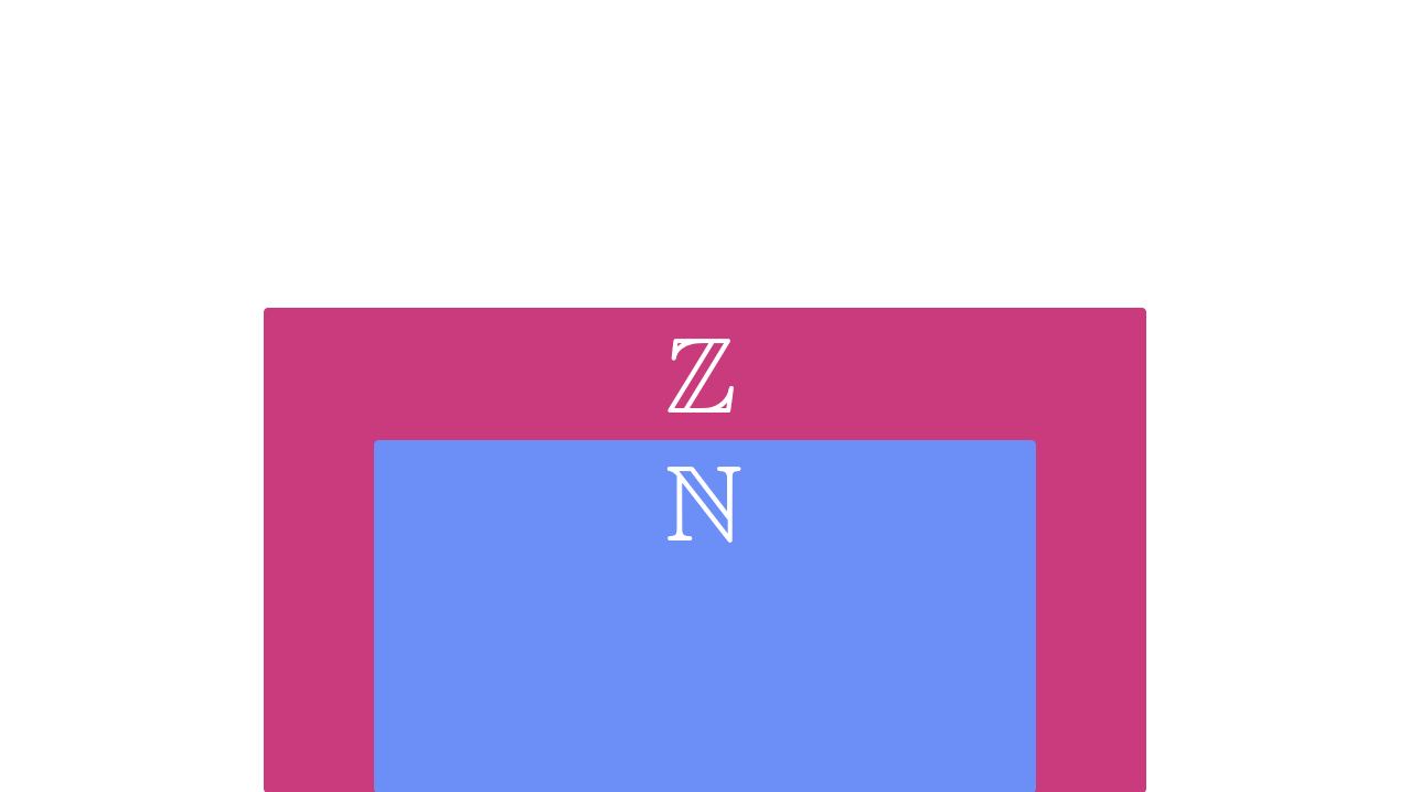
Figure 1.16 The number line with integers

Exercise 1.5   Write down the algorithms for arithmetic with \(\Z\). How are they similar to those for \(\N\)? How are they different?

Exercise 1.6   Determine whether \(\Z\) is closed under the four arithmetic operations we’ve covered thus far. Can you find an example that fails for any of them?

The additive inverse \(-n\) has extended our reach infinitely to the left on the number line. Not too shabby! I wonder what we’ll find by taking another look at multiplication.

Rational Numbers

Given \(n \in \mathbb{N}\), what do we multiply it with to get \(1\)? Last I checked, multiplication is an instruction to add repeatedly.

\(0 \times n = 0\) (don’t add anything)

\(1 \times n = 0 + n\) (add one copy of \(n\))

\(2 \times n = 0 + n + n\) (add two copies of \(n\))

\(-1 \times n = 0 + (-n)\) (negate \(n\) and add one copy)

Hmm. None of these examples seem like promising ways to get to \(1\). Since we’re talking about reversing processes, perhaps we can learn something useful from division.

\(n \div 0 = NO\) (undefined)

\(n \div 1 = n\) (break \(n\) into one piece)

\(n \div 2 = n\) (break \(n\) into two pieces)

\(n \div n = 1\) (break \(n\) into \(n\) pieces)

That last example is interesting. We got from \(n\) to \(1\)by dividing. I wonder if we could relate this to multiplication somehow. Time to play with notation a little.

\(n \div n = \frac{n}{n} = 1\)  

The new notation for division \(n/n\) is a fraction, or quotient. We know division produces a value, so let’s agree among friends that any time we see something like \(a/b\) it’s a number (unless \(b = 0\)).

The numbers we can write as quotients are known as the \(\mathbb{Q}\), the set of rational numbers. We could use set builder notation to express this idea concisely.

\(\mathbb{SET} = \{ elements \; \vert \; conditions \}\)  

The conditions required to build the set are known as the predicate. All together now.

\(\mathbb{Q} = \{ \frac{a}{b} \; \vert \; a,b \in \Z \; and \; b \neq 0 \}\)  

The rationals are my favorite set for a simple reason: I love pizza, I loved watching Teenage Mutant Ninja Turtles as a kid, and the Turtles LOVE their pizza.

Let’s say we have \(1\) pizza to share between \(n\) Ninja Turtles. What do we do? Easy! Just slice the pizza into identical pieces.

Figure 1.17 Pizza Time!

OK, you can divide a whole object into \(n\) pieces. And we agreed a moment ago that we could express such numbers as \(1/n\). So how many of those pieces does it take to reassemble the whole? Let’s stick with our pizza example for a moment longer.

\(\frac{1}{4} + \frac{1}{4} + \frac{1}{4} + \frac{1}{4} = 1\)  

That repeated addition looks an awful lot like multiplication!

\(4 \, (\frac{1}{4}) = 1\)  

It’s been quite the journey, but we’ve arrived at the multiplicative inverse \(1/n\). Given \(n \in \mathbb{N}\) and \(n \neq 0\),

\(n \, (\frac{1}{n}) = 1\)  

Figure 1.18 The sets \(\mathbb{Q}\), \(\Z\), and \(\N\)

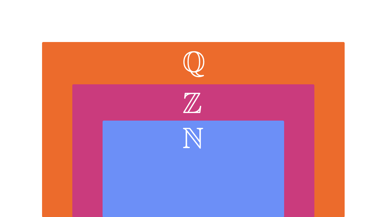
Figure 1.19 The number line with rationals

Exercise 1.7   How does \(\mathbb{Q}\) relate to \(\N\) and \(\Z\)? Is it a superset, a subset, or something else?

Exercise 1.8   Write down the algorithms for arithmetic with \(\mathbb{Q}\).

Exercise 1.9   Determine whether \(\mathbb{Q}\) is closed under the four arithmetic operations we’ve covered thus far. Can you find an example that fails for any of them?

Exercise 1.10   Does the multiplicative inverse work for \(n \in \Z\)? How about for \(n \in \mathbb{Q}\)?

Irrational Numbers

The gang’s all here, right? We’ve expanded the number line infinitely in both directions and figured out how to slice it up as needed. It certainly seems like we have everything we need to get started.

Well, almost. We started our journey with the operations addition, subtraction, multiplication, and division, but you may have noticed that I left somebody out: exponentiation.

\(n^{2} = n \cdot n\)  

A positive exponent is an instruction to multiply repeatedly, similar to how multiplication is an instruction to add repeatedly. Negative exponents also have a familiar feel; they are just instructions to divide repeatedly.

\(n^{-2} = \frac{1}{n^{2}} = \frac{1}{n \cdot n}\)  

The notation comes in very handy: try saying “repeat repeated subtraction” five times fast.

This new operation has even more in common with its predecessors. Addition and subtraction are inverses, meaning they undo each other.

\(0 + 5 - 5 = 0\)  

The same goes for multiplication and division.

\(1 \cdot 5 \div 5 = 1\)  

You can also invert an exponent by taking a root. For example,

\(\sqrt{3^{2}} = 3\)  

More generally, you would invert an exponent of \(n\) by taking the \(n\)th root.

\(\sqrt[n]{x^{n}} = x\)  

But let’s stick with the second root, or square root, for a bit. You could rewrite that first example as:

\(\sqrt{9} = 3\)  

This example happened to work out cleanly because \(9 = 3^{2}\). We call it a perfect square because we can “square” an integer to find it. Imagine creating a rectangular shape three blocks wide and three blocks high — a square.

Figure 1.20 Squaring three

Here are the first few perfect squares and their roots.

\(\sqrt{0} = 0\)  

\(\sqrt{1} = 1\)  

\(\sqrt{4} = 2\)  

\(\sqrt{9} = 3\)  

\(\sqrt{16} = 4\)  

OK, I have a question: are the sets we’ve covered thus far closed under square roots?

It turns out they are not. In fact, \(\sqrt{2}\) cannot be expressed in \(\mathbb{N}\), \(\mathbb{Z}\), or \(\mathbb{Q}\). There is no simple fraction \(a/b = \sqrt{2}\), so we call \(\sqrt{2}\) an irrational number.

Proof

You might ask, “What? No explanation?” Nope. You’re going to prove that \(\sqrt{2}\) is an irrational number. Or, more concisely, \(\sqrt{2} \in \mathbb{P}\).

\(\mathbb{P}\) is the set of irrational numbers: \(\{\sqrt{2}, e, \pi, ...\}\)

Proofs are structured arguments that mathematicians use to form the foundation of their science. This is your science now, too, so it’s time to run some experiments. The following examples are a warm-up for your own proof writing.

Let’s agree on the following definitions about parity.

An integer \(a\) is even if and only if \(a = 2j\) where \(j \in \Z\).

An integer \(b\) is odd if and only if \(b = 2k + 1\) where \(k \in \Z\).

In other words, all multiples of \(2\) are even, and all the integers in between the even integers are odd.

Alright, let’s go!

Theorem: Given \(a,b \in \Z\), if \(a\) is even and \(b\) is odd, then \(a + b\) is odd.

Proof: By definition, we know \(a = 2j\) and \(b = 2k + 1\). Then \(a + b = 2j + 2k + 1\).

The distributive property gives us \(2j + 2k = 2(j + k)\), so we can rewrite the expression as \(2(j + k) + 1\).

\(j + k\) produces an integer \(m \in \Z\), so the expression simplifies to \(2m + 1\), which is odd as required. \(\blacksquare\)

This was a proof by construction; we took a few definitions and marched directly toward the result. The \(\blacksquare\) at the end is a common way to end proofs. You may also see \(QED\) out in the wild, which stands for the Latin phrase “quod erat demonstrandum” or “what was to be shown”.

Instead of proof by construction, you could have easily taken another route. Let’s take the same definitions and try to develop an equivalent proof by contradiction.

Theorem: Given \(a,b \in \Z\), if \(a\) is even and \(b\) is odd, then \(a + b\) is odd.

Proof: By contradction. Assume \(a + b\) is even and write \(a + b\) as \(2m\) where \(m \in \Z\).

By definition, \(a = 2j\) and \(b = 2k + 1\). That means \(2j + 2k + 1 = 2m\).

The distributive property gives us \(2j + 2k = 2(j + k)\), so we can rewrite the expression as \(2(j + k) + 1\).

\(j + k\) produces an integer \(n \in \Z\), so the expression simplifies to \(2n + 1\), which is odd. This is a contradiction. \(2m\) is even and cannot equal \(2n + 1\).

Our assumption that \(a + b\) is even must be false. \(\blacksquare\)

Exercise 1.11   Prove \(\sqrt{2} \in \mathbb{P}\). Hint: use contradiction assuming \(\sqrt{2} \in \mathbb{Q}\).

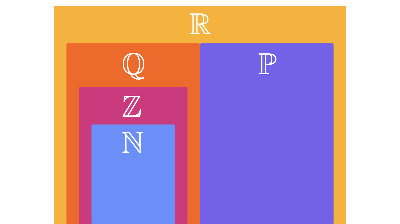
Exercise 1.12   Draw a diagram describing how \(\N\), \(\Z\), \(\mathbb{Q}\), and \(\mathbb{P}\) relate to each other.

Figure 1.21 The real number line

OK, we’ve covered natural numbers, integers, rational numbers, and irrational numbers. We now have arithmetic and the entire number line in our back pocket. Let’s see what we can do with this combined set of real numbers, \(\mathbb{R}\), by using it to explore the nighttime sky. I also think you’re ready to start visualizing things for yourself.

Figure 1.22 The set of real numbers, \(\R\)

1.2 Hello, p5

Now that you have a handle on numbers, let’s get you up and running with coding. A computer program is a set of instructions for your computer to follow, and coding is the process of writing down those instructions.

We will code in the JavaScript programming language using a “software sketchbook” called p5.js. This environment is designed with beginners in mind and makes it simple to create visual programs like the constellation you will simulate in a bit. Programs are called sketches in p5 lingo.

// Hello!
// This is computer code. Specifically, it is a comment just for you.
// Comments are notes for yourself or for other programmers.
// Lines of code that begin with // are comments.

Code editors such as the one below are embedded throughout the book so that you can explore ideas as they arise. If you would like to save your work, a great option is to follow along using the p5 Editor. You can use this code editor free of charge, with or without creating an account.

Example 1.1 Starter sketch

Exercise 1.13   Click the button, then click the button. What happened?

Let’s unpack this sketch a little.

In code, a function is a set of instructions that the computer can follow.

In the previous sketch, we know that you painted a canvas light gray. You did so by first defining the function setup(). The setup() function runs, or executes, once at the beginning of the sketch.

function setup() {
  // this code runs once
}

Each function bundles related instructions together under a common name and wraps them in curly braces {}. Let’s restore the full code from the previous example.

function setup() {
  createCanvas(200, 200) // didn't use 'function'
}

setup() uses, or calls, an existing function, createCanvas(), to create a drawing canvas. Note that we don’t use the keyword function when calling a function, only when defining one. Lucky for us, a team of programmers already figured out how to display a drawing canvas on your screen.

Those \(200\)s are inputs, or arguments, that determine the width and height of the canvas. Calling a function in most programming languages looks like the following.

doStuff() // no arguments
doStuff(argument) // one argument
doOtherStuff(argument1, argument2) // two arguments

Exercise 1.14   Change the arguments to createCanvas() to a different pair of numbers, then click the button again. What happened?

Color

OK, so you can change the dimensions of your canvas to whatever you like. How about changing the color? Let’s take another look at the draw() function.

function draw() {
  background(220)
}

draw() executes repeatedly in a loop that repaints the canvas about \(60\) times per second. The call to background() handles painting the canvas’ background. But what does 220 mean?

Grayscale

Your computer stores color in its memory as a sequence of binary digits, or bits. Think of bits as tiny switches with a value of either \(0\) (off) or \(1\) (on). Combining \(2\) bits gives us \(2^{2} = 4\) possible values (\(0\) and \(0\), \(0\) and \(1\), \(1\) and \(0\), \(1\) and \(1\)).

Table 1.1 All possible two-bit states

Combining 8 bits, or 1 byte, gives us \(2^{8} = 256\) possible values. p5 uses \(8\)-bit grayscale color, so we have \(256\) shades of gray at our fingertips.

Example 1.2 Working with grayscale

Exercise 1.15   Change the argument passed to background() to \(0\). What happened? Try a few different values between \(0\) and \(255\).

Named Colors

Grayscale is great, but it’s a little limited. There are several ways to work with color in p5, so our next stop is named colors.

p5 supports a large set of named colors that make quite the crayon box. You can choose from colors like fuchsia, limegreen, dodgerblue, and dozens more. The sketch below demonstrates how to paint your background dodgerblue by changing the argument passed to background().

Example 1.3 Using the crayon box

Drawing

Canvases painted one solid color have shown up time and again in the work of artists like those you’ll meet in the next chapter. For now, let’s continue our exploration of p5’s drawing capabilities by focusing on a single position, or point.

Drawing a point is as easy as calling the function point() with a pair of numbers as arguments. The sketch below draws a point in the middle of the canvas.

Example 1.4 Getting to the point

The result might be a little… confusing. Did anything happen? If you look closely, you’ll see a single, solitary point drawn at the center of your canvas.

Pixels

The canvas you created is \(200\times200\) picture elements, or pixels, wide and high. Imagine dividing your screen into squares like a checkerboard; each square is a pixel shining with a particular color.

The point you drew is \(1 \times 1\) pixels, so it’s like you drew it with a fine tip black pen. You can adjust the thickness, or weight, of your drawing by calling the strokeWeight() function with a number as an argument. And you can adjust the drawing color by calling the stroke() function with a named color as an argument.

Example 1.5 Swapping a pen for a marker

Exercise 1.16   Play around with the background color and stroke until you find a combination you enjoy.

You can draw additional points by calling the point() function again with different arguments.

Example 1.6 Adding points

Coordinates

In the Tron films, the Grid is the structure a digital world is built upon. We’ll create our own version in another tutorial. As a first step, let’s set up a coordinate plane using the grid of pixels on your screen.

Coordinates in two dimensions define position as an ordered pair of numbers \((x,y)\). The first number is the horizontal \(x\)-coordinate and the second number is the vertical \(y\)-coordinate. If you’ve played checkers or used graph paper, then you’ve got the idea.

The first point you drew at \((100,100)\) wound up at the center of your \(200 \times 200\) canvas. Coordinates describe individual positions, or points on the drawing canvas. Coordinates are given relative to the point \((0,0)\), called the origin. In our sketchbook, the origin is located at the top-left corner of the drawing canvas.

Take a break from the computer and open up your favorite book to its first page. Where on the page would you start reading?

My favorite book thus far is Slaughterhouse-Five by Kurt Vonnegut. It was originally written in English, a Western language in which you start reading near the top-left corner and move straight across the page to the right. At the end of each row of letters, you return to the left of the page. Then, you move down one row to continue reading.

This pattern is similar to the coordinate system used in our sketchbook: \(x\) increases from left to right and \(y\) increases from top to bottom.

Exercise 1.17   Draw some points at \((0,0)\), \((50,100)\), and a few other coordinates. What happnes as you increase and decrease \(x\)-coordinates? How about \(y\)-coordinates?

1.3 Constellation

Your computational toolkit is growing quickly, so let’s put it to use by creating our first system. The systems I refer to in this book are sets of related objects that we can 1) model using mathematics and 2) simulate using computers. It’s a broad definition with many applications we’ll explore together.

For starters, let’s look to the heavens and define a system. Defining a system sets the bounds of what you want to simulate. You only need to be specific enough to be productive. There’s no need to write an essay when a sentence or two will do!

  A constellation in the nighttime sky.

Now comes the tricky part: we need to frame the system in such a way that you can describe it using mathematics. The simplest representation, or model, I can think of is to treat the whole sky as empty space with a few points of light strewn across it.

\(\mapsto\)   Outer space is an empty, infinite, two-dimensional surface. Stars are points of light within this plane.

Two-dimensional space is made up of infinitely many \((x,y)\) coordinate pairs where \(x,y \in \mathbb{R}\). Your computer is limited in terms of memory and processing power, so there are limits to how many numbers it can represent. We’ll use JavaScript’s floating point numbers, which are numbers with decimal places, to represent coordinates. The set of floating point numbers isn’t infinite like \(\mathbb{R}\) but it’s large enough to get us started. These floating point coordinates will be our first set of information to process, otherwise known as data.

  Star coordinates are ordered pairs of floating point numbers.

Table 1.2 The “Little Bear” data set

We now have a pretty clear idea of what we’d like to draw, but the how is still missing. There’s quite a bit going on behind the scenes in p5, but we can safely ignore most of those details. The algorithm for this simulation is fairly simple.

  First, paint the night sky. Then select a pencil color & weight. Finally, draw a point at each star’s position.

And voilà! You’ve designed your first system. Let’s code it up.

Exercise 1.18   Research your favorite constellation or make one up. Adjust the stroke before drawing each point of light in order to match its size and color.

Now that we have a working system, let’s study it. Here’s my first question: how much space does this constellation take up in the sky?

Domain and Range

Many patterns and relationships are difficult to see when written as a bunch of numbers. You can visualize any mathematical idea or data set, and doing so is often illuminating. The constellation you drew using the data in Table 1.2 is not just a quick piece of art. It also doubles as a special type of mathematical diagram called a graph.

Figure 1.23 “Little Bear” on graph paper

Discrete Graphs

The entire set of points makes up a disconnected, or discrete, graph. The set of \(x\)-values, called the domain, is \(\{20,55,90,125,150,175\}\). We usually write the elements of a set in increasing, or ascending, order. The set of \(y\)-values, or range, is \(\{85,100,115,120,127,130,135\}\).

Exercise 1.19   Write down the domain and range of the stars in the discrete version of your constellation.

Continuous Graphs

What happens when we connect the dots? You can draw a line between two points by calling the function line() with four arguments: the \(x\) and \(y\)-coordinates of the starting point and the \(x\) and \(y\)-coordinates of the ending point.

Example 1.7 Connecting the dots

Exercise 1.20   Our constellation doesn’t look quite finished. Add a few calls to the line() function to connect the stars in your constellation.

If you zoom in and move from the lowest \(x\)-values to the highest, you would find that the graph is filled in somewhere at every \(x\)-value between \(20\) and \(175\). You could do the same from the lowest \(y\)-values to the highest. When a graph’s domain and range take on every value within an interval, we say it is continuous.

We can describe the continuous domain and range concisely using the inequalities \(>\), \(<\), \(\ge\), and \(\le\). The expression \(2 > 1\) means “\(2\) is greater than \(1\).” \(3 \le 3\) means “\(3\) is less than or equal to \(3\)”. And \(4 \le x \le 5\) means “\(x\) is greater than or equal to \(4\) and \(x\) is less than or equal to \(5\).”

In the “Little Bear” example, the domain is \(20 \le x \le 175\) and the range is \(85 \le y \le 135\).

You can account for any gaps in your domain and range by listing each interval separately. For example, imagine you saw the set of stars we’ve discussed a little differently than the ancient astronomers did.

Example 1.8 Think different

Now there is a gap in the domain between \(90\) and \(125\). You could express the new domain as \(20 \le x \le 90\) or \(125 \le x \le 175\). And the range? The graph is still filled in somewhere between \(85\) and \(130\), so it’s still \(85 \le y \le 130\).

Exercise 1.21   Write down the domain and range of the stars in the continuous version of your constellation.

Exercise 1.22   What is one thing you like about your constellation? What is one thing you would change?

1.4 Meteor

Curiosity is one of my favorite attributes of people. As small children, we constantly run experiments to make sense of our world. We never really stop. Humans have both purposely searched for patterns and intuitively identified relationships throughout our history. But it’s only in the last couple of millennia that we’ve applied formal structure to this pursuit, and that structure has made all the difference.

Over the last few sections, you studied real numbers and used them to simulate a distant constellation. But what if we tried exploring a system that’s a little closer to home, like a meteor skimming across the sky?

Variables

Our original model of a star as a fixed point of light won’t cut it for a shooting star. Quantities that change, like the position of a meteor, are known as variables. In code, you would create a variable as follows.

Example 1.9 Declaring and assigning a variable

Line 8 of the sketch declares the variable x and assigns it the value 100 using the assignment operator =. Think of this as asking the computer, “Would you please give me a box labeled x and put 100 in there?”

Running this sketch isn’t so exciting; we just have another point sitting in the middle of the canvas. Each time draw() executes, the memory containing x is cleared before another copy is created and assigned the value 100. But wait! We we can also declare the variable x up top in the global scope. By doing so we can

1. Access x anywhere in the sketch and
2. Modify x across calls to draw().

For starters, how about we increase, or increment, x each time the canvas is painted?

Example 1.10 Using global variables

This is a pretty big moment. You just implemented linear motion! Let’s describe our new meteor simulation.

  A meteor in the nighttime sky.

\(\mapsto\)   Outer space is an empty, infinite, two-dimensional surface. A meteor is a point of light traveling along a straight path.

  The meteor’s coordinates are ordered pairs of floating point numbers. Its initial position is \((0,200)\).

  First, paint the sky. Next, select a pencil color & weight. Then, update the meteor’s position. Finally, draw a point at the meteor’s position. Repeat.

This algorithm still seems a little mysterious, so let’s clarify a bit. The addition assignment statement on line 11 asks your computer, “Would you take a look at the value stored in x, add 1 to it, and store that instead?”

But even if the addition assignment operator += does the job I just described, why does the meteor continue moving? Recall that draw() executes each statement that’s indented underneath it from top to bottom about \(60\) times each second.

You could track the effect of line 14 by calling the text() function to display the variable x after each update. Have a look at the function’s documentation to learn more about how it works.

Example 1.11 Displaying values

Exercise 1.23   Change the initial value of x from 100 to something else. Then, change the increment on line 11 to some number other than 1.

Exercise 1.24   What does the -= operator do?

Linear Equations

OK, you’ve got things moving. Now imagine looking up one night to see a meteor streak across the heavens. What are the odds it’s traveling precisely left to right, parallel to the horizon? Probably somewhere near zero. I think we need to expand our modeling toolkit a little.

You already know how to update the value of your meteor’s \(x\)-coordinate. Let’s use a similar technique to update the \(y\)-coordinate, but this time we’ll establish a relationship between \(x\) and \(y\). For starters, let’s have \(y\) follow \(x\) exactly.

Example 1.12 A linear relationship

In mathematics, equations establish relationships between one or more variables. Line 12 could be written as the following linear equation.

\(y = x\)  

When \(x\) changes on the right, \(y\) must change on the left in order to maintain equality. If \(x\) increases by \(1\), so will \(y\). But you aren’t limited to just mirroring values! Linear equations let you multiply, or scale, the variable \(x\) by a number like so.

\(y = 2x\)  

Now, when \(x\) in increases by \(1\), \(y\) increases by \(2\). You can also add an offset, or translate, the graph.

\(y = 2x + 5\)  

You can describe straight lines in general by writing them in slope-intercept form:

\(y = mx + b\)  

where \(m,b \in \mathbb{R}\). We call \(m\) the equation’s slope and \(b\) its \(y\)-intercept. Let’s experiment a little with \(m\) and \(b\) in code using the addition + and multiplication * operators.

Example 1.13 Coding linear equations

Exercise 1.25   Try different values for your slope and \(y\)-intercept until you find a combination that you like.

Exercise 1.26   Change the statement background('midnightblue') to background(25, 25, 112). Then, change it to background(25, 25, 112, 10). What happened? Read the documentation for the background() function and experiment a little.

Exercise 1.27   Extend your meteor simulation to include more objects from the nighttime sky. What is the system? What mathematical model(s) do you need to describe its behavior? What data are involved? And what algorithm(s) do you need to make it run?

Exercise 1.28   Start a new simulation from scratch. Will it be a rainstorm? Or a swarm of bugs? As you get started, describe the system, its mathematical model(s), its data, and the algorithm(s) that make it run.

Exercise 1.29   What is one thing you found challenging about building your own simulation? What is one thing you enjoyed?

Believe it or not, linear equations like the ones you just created are key to everything that follows in these tutorials. In the next tutorial, we’ll combine several of these equations into a linear system.

Reference

• Intermediate Algebra 2e / Chapters 1–3
• Precalculus / Chapters 1–2

This work is licensed under a Creative Commons Attribution-NonCommercial-ShareAlike 4.0 International License.