Tutorial 3. Functions

Wait, they don’t love you like I love you
Wait, they don’t love you like I love you
Maps
Wait, they don’t love you like I love you

— “Maps” by Yeah Yeah Yeahs

Over the last two tutorials, you used equations to establish relationships between variables. We’re going to build on those ideas in this tutorial as you acquire one of the most powerful tools in computation: abstraction.

3.1 Maps

Input/Output

Many of the systems we’ll study together take some kind of input and produce an output. Let’s consider a familiar example: a toaster. A toaster takes a slice of bread as its input, applies heat, and produces a toasted slice of bread as its output. Mathematicians like us call this sort of input/output process a map or function.

Figure 3.1 Transforming bread into toast

Bread entering and exiting a toaster

A bit more formally, a map applies a rule to assign elements from a set of inputs to a set of outputs. The set of inputs is called the map’s domain and the set of outputs is called its range or image.

Let’s see this input/output process in action with a concrete example. I’m going to flip a coin. You win if the coin lands on heads and you lose if it lands on tails.

$H \mapsto Win$

$T \mapsto Lose$

The $\mapsto$ is a common shorthand for “maps to”. In this example, the domain is the set $\{H, T\}$ and the range is the set $\{Win, Lose\}$. Our simple game is based on a rule that assigns the result of a coin flip to an outcome. Inputs map to outputs. It’s a perfectly valid map despite its lack of numbers. All we need is a rule!

You could also represent the same map as a set of ordered pairs of inputs and outputs. I’ll organize the ordered pairs neatly in a table.

Table 3.1 A tabular representation of a coin flip

Coin Side	Game Result
Heads	Win
Tails	Lose

Now, I’ll define another rule, called $d$, using notation that we’ll use throughout the rest of the book. There is nothing special about the name $d$; any letter will do just fine. In the equation below, $d$ is the doubling function; it takes a numerical input $x$ and multiplies it by $2$ to produce its output $d(x)$.

$d(x)=2x$

Figure 3.2 Parts of a function

Parts of a function

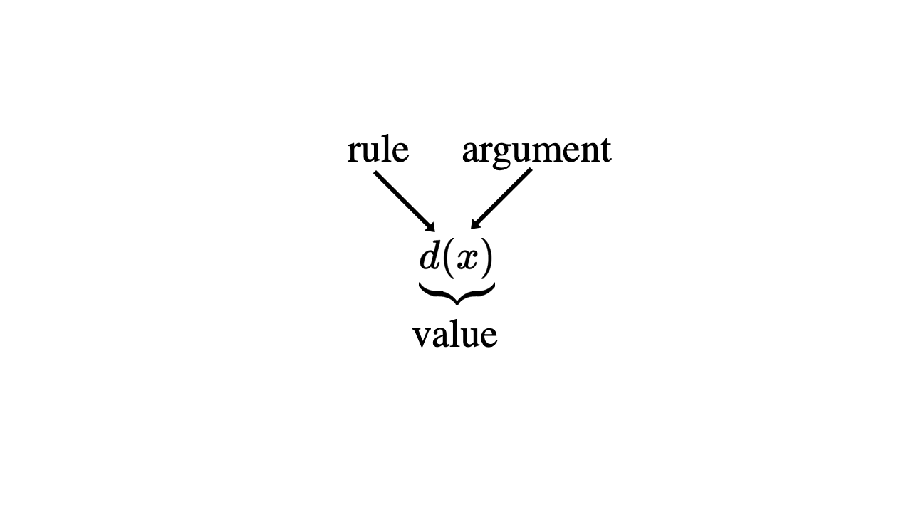
In the diagram above, $x$ is an element of the function’s domain. The rule $d$ is applied to x to produce $d(x)$, an element of the function’s range. $x$ is the argument provided to $d$ and $d(x)$ is the resulting value.

Figure 3.3 Mapping values from the domain to the range

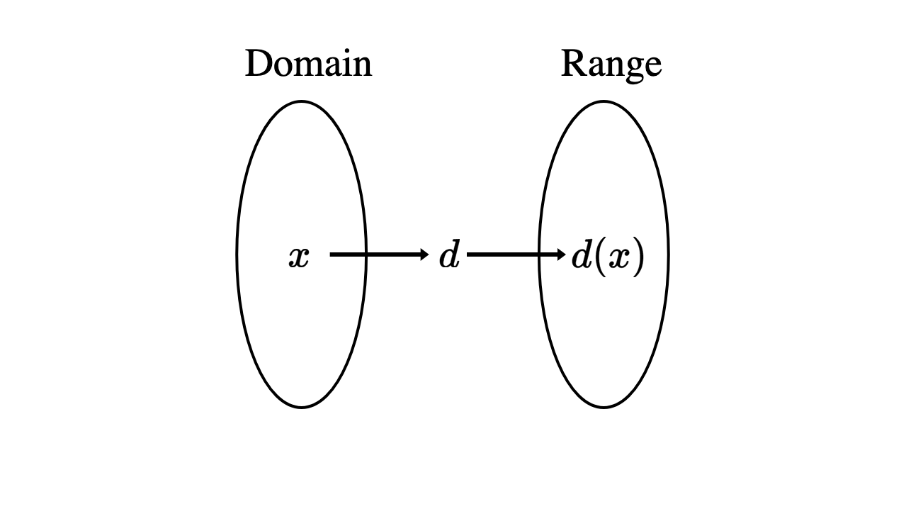
Mapping values from domain to range

Now that we have a rule, let’s apply it to an argument of $3$. We also call this process evaluating the function for the argument $3$.

$d(3)=23$

$d(3)=6$

So, the value produced by evaluating $d(3)$ is $6$. The doubling function $d$ is a specific example of a linear function. Linear functions multiply their argument by a number and then add another number to the value produced from multiplication. You can represent linear functions in the familiar form of a linear equation.

$f(x)=mx+b$

$f$ is the most common name for functions, but again, any letter will do. In the doubling function, $m=2$ and $b=0$.

$d(x)=2x+0$

Equations Interlude

Functions and equations share some notation as we just saw, but they are distinct concepts. The linear equation

$y=2x+5$

looks an awful lot like the linear function

$g(x)=2x+5$

However, keep in mind that a function describes a mapping from inputs to outputs. It is a one-way process, and we even denote it with the “maps to” arrow to point this out.

$x \mapsto g(x)$

You can describe the same function in any way that conveys the rule. For example, you could create a table of arguments and their corresponding values as we did with the coin flip. Here is part of the table representing $g$.

Table 3.2 A tabular representation of $g$

$x$	-1	0	1	2
$q(x)$	3	5	7	9

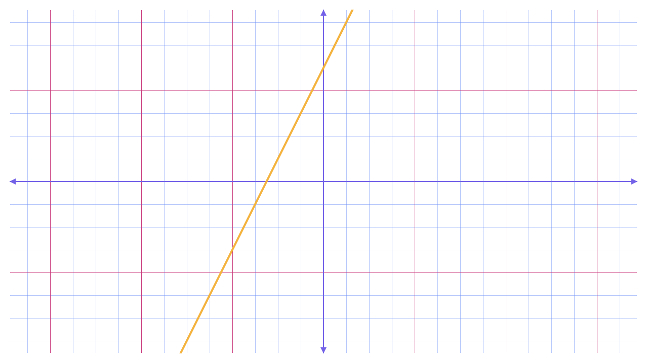
In addition to equations and tables, there is also the graph of $g$. You can generate a visual representation for a function by thinking of the values of $g(x)$ as $y$-coordinates. Now the task simply requires drawing a point at each coordinate pair $(x,g(x))$.

Note that graph below uses a coordinate system more common in math class; namely, the $y$-axis points up. Moving between coordinate systems takes a bit of getting used to, but this mental will serve you well as you explore more coordinate systems in the future.

Figure 3.4 A graphical representation of $g$

A straight line

OK, we’ve seen three ways to represent functions: a formula expressed as an equation, a table of input/output pairs, and a graph of inputs and outputs. One of these representations is built around an equation, while the others are not.

As we saw in the last tutorial, equations can be rearranged and solved in a variety of ways that may have nothing to do with input or output. An equation is a statement of equality that specifies a relationship, nothing more. Functions and equations overlap a little, but they are distinct concepts.

Domain and Range

Functions can be as simple as doubling or as complex as you like. When given a rule, it’s often helpful to know when it applies and when it doesn’t. Let’s take a look at a new rule $q$ I’ll call a quadratic function, which means it involves squaring a number.

$q(x)=x^{2}$

The set of real numbers is closed under multiplication, and $q$ just multiplies its argument by itself, so we could take any real number and use it to evaluate $q$ to produce a value. That means the domain of $q$ is the set of real numbers.

Domain: $\mathbb{R}$

We can build up a little intuition for how this function behaves by evaluating it for a small subset of the real numbers.

Table 3.4 A tabular representation of $q$

$x$	-2	-1	0	1	2
$q(x)$	4	1	0	1	4

Interesting. There seems to be a sort of symmetry in the table representing $q$. I wonder what this looks like when graphed.

Figure 3.5 A graphical representation of $q$

A parabola

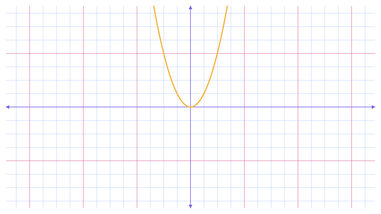
That U-shaped graph is known as a parabola. We’ll get to know it much better in the next tutorial, but we can already observe some key details. Between the table and the graph, it’s clear that $q$ never produces a value below $0$. In other words, its range is the set of positive real numbers and $0$.

Range: $q(x) \ge 0$

Let’s look at one more rule together which I’ll call a square root function.

$s(x) = \sqrt{x}$

$s$ stakes its argument $x$ and produces a value which, multiplied by itself, equals $x$. Something strange happens when we start evaluating $s$ for the same subset of the real numbers.

Table 3.5 A tabular representation of $s$

$x$	-2	-1	0	1	2
$q(x)$	ERROR	ERROR	0	1	4

Let’s examine what happens when we evaluate $s(-1)$. The rule $s$ tells us to compute the number which, multiplied by itself, equals $-1$. The first possibility that comes to mind is $-1$, but $-1 \times -1=1$, not $-1$ as required. And $1 \times 1$ is also $1$. We’re stuck!

There is no real number that we can multiply by itself to produce $-1$. Take a moment to prove that multiplying two numbers with the same sign always produces a positive number.

Bringing this back to the rule $s$, we don’t have any sensible way to evaluate it for negative inputs. That means we need to restrict its domain to the real numbers greater than or equal to $0$.

Domain: $x \ge 0$

Now I’m curious to see what this function looks like when graphed.

Figure 3.6 A graphical representation of $s$

Half of a parabola

Just as we saw with $q$, it’s clear that s never produces a value below $0$. Its range is also the set of positive real numbers and $0$.

Range: $s(x) \ge 0$

We just demonstrated that the set of real numbers isn’t closed under taking square roots. This problem will be our jumping off point for generating fractals in the next tutorial.

Exercise 3.1 Find the domain and range of $a(x)=2x+5$

Exercise 3.2 Find the domain and range of $b(x)=(x-3)^{2}+4$

Exercise 3.3 Find the domain and range of $c(x)=\sqrt{x+1}-7$

Inverses

In the first function we studied together, a coin flip resulted in one of two possible outcomes. If you told a friend that you had just won the coin flip game, it would be easy for them to work backwards and figure out what had happened; the coin must have landed on heads.

Working your way from an output back to an input is known as inverting a function. Some rules, like our coin flip game, are easy to invert.

$H \gets Win$

$T \gets Lose$

But other rules aren’t so clear. Let’s play another game of chance, this time with a pair of dice.

Figure 3.7 A six-sided die

Six faces of a die

Each face of a die has a value from $1$ to $6$ corresponding to the number of segments on the face. When you roll a die, its value is the face pointing up. You win the game if you roll a pair of dice with values that sum to an even number, and you lose if they sum to an odd number.

$Even \mapsto Win$

$Odd \mapsto Lose$

The game is afoot! How many ways are there for you to win?

We can represent each dice roll using an ordered pair of numbers like $(1,3)$ or with a picture. I’ll keep the analysis manageable by considering dice rolls of $(1,3)$ and $(3,1)$ as the same roll.

Figure 3.8 The set of winning combinations of dice

Dice pairs with even sums

There are so many ways for you to win! If you did win, and you shared the news of your win with a friend, they would have no idea whether you rolled $(1,1)$ or $(4,6)$ or some other combination of dice that sum to an even number. There is no clear path from an output back to a unique input.

$(1,1) \gets Win$

$\vdots$

$(4,6) \gets Win$

$\vdots$

$(6,6) \gets Win$

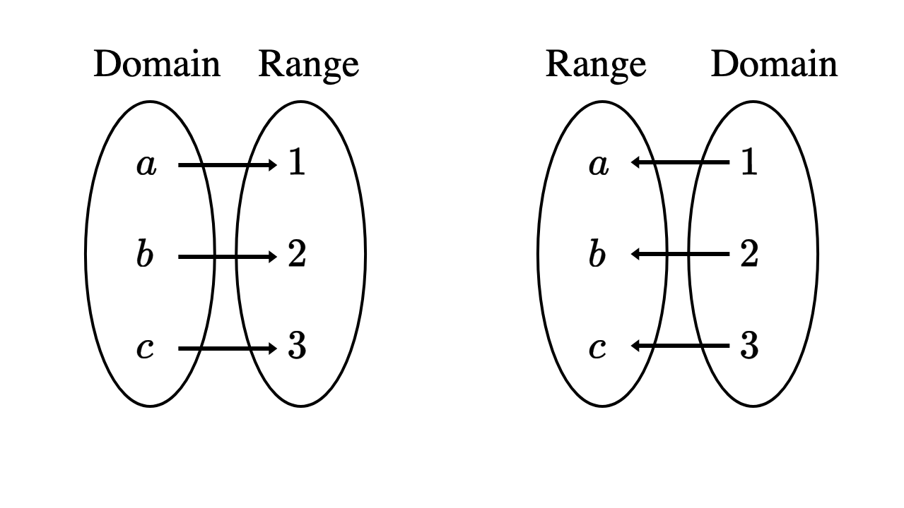
Unlike the coin flip, the dice role is not invertible. A function is only invertible if each element of the domain maps to a unique element of the range. This is also known as a bijective map.

Figure 3.9 A function and its inverse

A mapping and its inverse

The process of inverting a function depends on the representation you’ve chosen for it, but the idea is always the same: your inputs and outputs are reversed. Let’s take another look at the function $g(x)=2x+5$.

Table 3.6a A tabular representation of $g$

$x$	-1	0	1	2
$g(x)$	3	5	7	9

The inputs in the left-hand column correspond to outputs in the right-hand column. Inverting this table simply requires swapping the two columns. The inverse of a function like $g$ is typically written $g^{-1}$ which is read “$g$ inverse”.

Table 3.6b A tabular representation of $g^{-1}$

$x$	3	5	7	9
$g^{-1}(x)$	-1	0	1	2

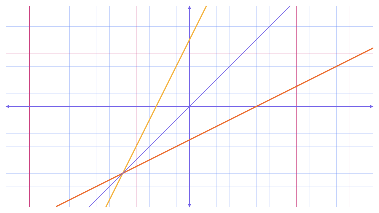
The visual result of inverting a function is striking for its symmetry. Inputs and outputs are swapped, so the corresponding $x$ and $y$-coordinates are also swapped.

Figure 3.10 A graphical representation of $g$ and $g^{-1}$

A pair of intersecting lines with symmetry

Inverting a function represented as an equation also involves swapping and reversing. Let’s continue with our old friend $g(x)=2x+5$. The mathematical operations that comprise equations follow a specific order, so it’s straightforward to run those operations in reverse.

I’m going to subvert standard notation a little bit and rewrite the function as follows:

$g=2x+5$

Now let’s swap the input $x$ and output $g$.

$x=2g+5$

That’s actually all there is to inverting a function represented as an equation. But now it’s not clear how an input $x$ is supposed to produce an output; this rule isn’t easy to follow. We can clarify the process by solving the equation for $g$.

$x-5=2g+5-5$

$x-5=2g$

$\frac{x-5}{2}=\frac{2g}{2}$

$\frac{x-5}{2}=g$

The last step is to tidy up our notation. We just inverted $g$, so this final equation represents $g^{-1}$.

$g^{-1}(x)=\frac{x-5}{2}$

$g^{-1}(x)=\frac{1}{2}x-2.5$

Inverting a function represented as an equation involves two steps. First, swap your input and output variables. Second, solve the equation for the output variable. The second step may require a fair amount of algebra, and it’s easy to get lost in a jungle of symbols. Keep in mind that inverting involves swapping and reversing.

Let’s take $r(x)=(x-3)^{2}+4$. First, rewrite for convenience.

$r=(x-3)^{2}+4$

Next, swap the input and output variables.

$x=(r-3)^{2}+4$

Following the order of operations, PEMDAS, that $+4$ would normally be the last operation applied. We’ll undo, or invert, that last operation first.

$x-4=(r-3)^{2}+4-4$

$x-4=(r-3)^{2}$

And now we’ll continue in reverse, working our way in toward the output variable, $r$, inverting operations along the way.

$\sqrt{x-4}=\sqrt{(r-3)^{2}}$

$\pm \sqrt{x-4}=r-3$

$\pm \sqrt{x-4}+3=r-3+3$

$3 \pm \sqrt{x-4}=r$

Last but not least, let’s rewrite this equation using our notation for inverses.

$r^{-1}(x)= 3 \pm \sqrt{x-4}$

That $\pm$ operation reads “plus or minus”. If we evaluate $r^{-1}(5)$, then the outputs are $2$ and $4$. Interesting. I wonder what that means in terms of the invertibility of $r$. You’ll examine $r$ and $r^{-1}$ more closely in Exercise 3.5.

Functions are a one-way process and some functions can run in reverse just fine. Others cannot. Thinking back to our toaster metaphor, you can run bread through a toaster to make toast, but there isn’t an anti-toaster to revert the toast back to its pre-toasted existence.

Exercise 3.4 Determine whether the function $h$, represented in tabular form below, is invertible.

$x$	-2	-1	0	1	2
$h(x)$	4	1	0	1	4

Exercise 3.5 Determine whether the function $r(x)=(x-3)^{2}+4$ is invertible. If so, find the equation of its inverse $r^{-1}$ and check your work against the example above. If not, explain why it isn’t invertible in plain English.

Exercise 3.6 Determine whether the function $s(x)=\sqrt{x+1}-7$ is invertible. If so, find the equation of its inverse $s^{-1}$. If not, explain why it isn’t invertible in plain English.

3.2 JavaScript Functions

Functions are a big deal in mathematics–so big that their study led to the founding of computer science. It’s no coincidence that every major programming language has a way to define mathematical functions like the ones we just discussed. Let’s explore how functions work in JavaScript and begin defining our own.

Following Procedures

In code, functions bundle together a sequence of instructions, or statements, and give them a name. Organizing our code with functions enables us to work at a higher level of generality, or abstraction, than we could otherwise. Doing so can make it easier to plan our programs and to analyze them, whether to improve performance or to fix errors that inevitably crop up. They also enable programmers to share their solutions to problems so that others can build upon them.

You can define functions to do almost anything imaginable, from solving important math problems to creating delightful multimedia experiences. As tiny computers are increasingly embedded into a wider range of products, the ability to control computers is approaching the sort of witchcraft and wizardry normally reserved for fantasy novels.

The sketches you’ve written so far all defined two functions: setup() and draw(). And nearly all of the code you’ve written has been part of the body of one of these two functions.

The function keyword begins a function header, which is the first line of code in a function’s definition. p5 looks for your definitions of setup() and draw() to figure out how to proceed once you press the play button. Much goes on behind the scenes to present a simple set of variables and functions that comprise p5’s application programming interface (API). Here is the subset of the p5 API you’ve used thus far along with links to the documentation for each variable or function.

Environment
width
height

Setting
background()
fill()
noFill()
noStroke()
stroke()

2D Primitives
line()
point()

Structure
setup()
draw()
noLoop()

Loading & Displaying
text()

We know that your statements are executed in order from top to bottom; this is the typical flow of execution in a computer program. When you call a function such as background() or point(), your program jumps over to the definition of the function and begins executing statements in the function’s body in order from top to bottom. Once finished, your program jumps back out of the program and picks up where it left off.

function setup() {
  createCanvas(200, 200)
}

function draw() {
  background(220) // jumped over to the definition of background
  // ... and we're back
  point(100, 100)
  // ...
}

Let’s revisit our first simulation of a constellation and tidy it up a bit using functions. I think we can break the simulation into two core pieces: drawing outer space and drawing stars. The process of taking a problem and breaking into simpler pieces is known as decomposition.

Example 3.1 Decomposing a constellation

It is much easier to keep track of what’s going on in your programs when you write code with descriptive names like drawConstellation(). We’ll use the JavaScript community’s convention of naming new functions and variables with multiple words separated by capitalization as opposed to spaces. In this naming convention, called “camelCase”, the first word is all lowercase and subsequent words begin with a capital letter.

Exercise 3.7 Rewrite one of your previous sketches and organize it using new functions you define. It may not be obvious at first how to delineate between different parts of your code, and there are probably multiple ways to do so elegantly.

Exercise 3.8 Rewrite one of your previous sketches and organize it using new functions you define. It may not be obvious at first how to delineate between different parts of your code, and there are probably multiple ways to do so elegantly.

Input/Output

The functions we’ve defined thus far do a nice job of bundling instructions together and organizing code, but they’re a bit limited. You can customize a function by adding a required input, or parameter, to its header. Let’s add a parameter to the drawConstellation() function.

function drawConstellation(starColor) {
  stroke(starColor)
  strokeWeight(3)
  point(20, 120)
  point(55, 130)
  point(90, 127)
  point(125, 115)
  point(150, 135)
  point(150, 85)
  point(175, 100)
}

Now, you can specify what color you want to draw your constellation by providing an argument when you call the function.

Arguments are assigned to parameters, and you can have more than one! For example, you could write a version of drawConstellation() that lets you specify the color and size of stars that are drawn.

function drawConstellation(starColor, starSize) {
  stroke(starColor)
  strokeWeight(starSize)
  point(20, 120)
  point(55, 130)
  point(90, 127)
  point(125, 115)
  point(150, 135)
  point(150, 85)
  point(175, 100)
}

Now you can customize the size and color of stars when you call drawConstellation().

Parameters are part of a function’s definition and only exist within a function’s body. The region of a program where a variable exists is called its scope. In our drawConstellation() example, the rest of the sketch has no idea what starSize means. Any variables you declare inside of a function are also invisible to the outside world; their scope is the function body. Let’s revisit one of our abstract paintings from the last tutorial and tidy up the code a little.

Example 3.2 Decomposing an abstract painting

The variables x and y only exist inside the body of the paintCanvas() function. They are examples of local variables, meaning they only exist locally inside of the function where they were created.

By contrast, variables you declare at the top of your sketch are visible throughout your code and are known as global variables. The meteor sketch was our first encounter with variables in the global scope.

Example 3.3 Revisiting global variables

It’s convenient for us to define the variables x and y in the global scope since we’re referring to the same meteor when we draw it and when we update its position.

Global variables can be helpful when used sparingly, but they can be hard to keep track of as your programs grow in size. It’s often better practice to produce, or return, values on the fly and assign them to local variables. Let’s see this in action with the collision example from the last tutorial.

Example 3.4 Introducing mathematical functions

The millis() function on line 6 is like a stopwatch built into p5; it returns the number of milliseconds that have passed since a sketch started its execution. We can use it to increase the value of x locally instead of globally.

The JavaScript functions s() and d() are equivalent to the mathematical functions $s(x)=0.5x+50$ and $d(x)=-0.5x+150$, respectively. When you call either function with an argument, they assign the argument to the parameter x and use x to compute a return value.

On line 7 of the previous example, it may seem strange to call s() with an argument x when `x. also happens to be the name of the function’s parameter Aligning variable and parameter names in this way can be helpful to clarify your intent, but it isn’t required.

Also on line 7 above, note that the value returned from s(x) is assigned the y parameter of drawShuttle(). Using the return value from one function as the argument for another is known as composition; we’ll discuss the idea in more detail in the next section. For now, let’s draw some more images.

Graphing with p5

Let’s continue drawing with functions by visualizing them as a set of points. Keep in mind that the $y$-axis points downward in computer graphics by default.

Example 3.5a Drawing a set of points

I can see the basic shape of the graph, but what gives with all of that empty space? Let’s draw the points a bit closer together by decreasing the value of our increment dx.

Example 3.5b Bonus points

Much better. But what if we changed the shape of the graph a bit by changing the value of a?

Example 3.5c Back to square one

Oof, the points on the graph are once again separated by empty space. We can continue adjusting the value of dx each time we draw a graph, but I think this is a nice opportunity to present another one of p5’s drawing capabilities: shapes. More precisely, we can connect a set of points, called vertices, using line segments to create a polygon. The following sketch draws the simplest polygon, a triangle.

Example 3.6a A triangle

This object isn’t quite a polygon, however, because the vertices don’t enclose a region of space. You can connect the final and initial vertices by adding the CLOSE argument to endShape().

Example 3.6b An enclosed triangle

p5 fills the interior of shapes with the color white by default. You can set the fill color for shapes by calling the fill() function like so.

Example 3.6c A colorful triangle

Back to our graph, let’s try to make our code more flexible by swapping out individual points for vertices connected by tiny line segments. That way, we are guaranteed to cover any gaps introduced by changing the graph’s shape. We aren’t concerned with the area enclosed by the graph just yet, so we won’t add the CLOSE argument to endGraph().

Example 3.7 Graphing with line segments

The variable width keeps track of the width of the drawing canvas; height keeps track of its height.

You could make the sketchbook function a little more like a graphing calculator by removing the default fill from the shape you just created. To do so, add a call to noFill() at the beginning of your graph() function.

function graph() {
  noFill()
  beginShape()
  // add vertices...
}

It’s worth taking a moment to present another loop syntax that can help to clarify our code. In the previous example we wrote the following:

let dx = 1
let x = 0
while (x < width) {
  vertex(x, f(x))
  x += dx
}

Let’s focus on the basic structure of the loop by removing the variable dx and the call to vertex():

let x = 0
while (x < width) {
  // do stuff
  x += 1
}

This steady, sequential increment has shown up repeatedly in our sketches. It turns out that the pattern can also be expressed using a for loop.

for (let x = 0; x < width; x += 1) {
  // do stuff
}

The loop header now completely describes the iteration. Start from $0$, stop at $200$, and count by $1$’s. When you know that your loop is meant to repeat a specific number of times, for loops can help to clarify that intent.

By way of contrast, while loops are especially useful when you aren’t sure how many iterations a process may need to complete.

while (stillLearning) {
  learn()
}

OK, let’s put for loops to work drawing graphs.

Example 3.8 Drawing a graph with a for loop

Exercise 3.9 Simulate a ball flying through the air along a parabolic path. Use a mathematical model like $f(x)=a(x-h)^{2}+k$ to describe the ball’s motion. Try setting a to a small negative number and choose a point $(h,k)$ as the peak of its flight. Decompose your simulation into a few functions including one that returns a value. The following code snippet may be a helpful template for describing your ball’s path.

function f(x) {
  let a = 0
  let h = 0
  let k = 0
  return a * (x - h) ** 2 + k
}

3.3 Combination and Composition

We’ve seen that mathematical functions are useful for modeling all sorts of phenomena, and that they are easy to express in a way that computers can execute. In this section, we’ll use financial modeling to explore a few ways that functions can work together.

Combination

Adding Functions

Given a pair of functions, it’s simple to combine their outputs using an arithmetic operation. Let’s say you invest in a pair of companies by buying shares of their stock and becoming a part-owner. The stock price of the first company, Acme Corporation, is currently $\$ 100$ and increases $7 \%$ annually, which we can express with the function $A(t) = 100 \cdot 1.07^{t}$. In this equation, $A(t)$ is the price of one share $t$ years after you bought the share for $\$ 100$. The second company, Whitewhale Consolidated Interests, also has a stock price modeled using an exponential function, in this case $W(t)=80 \cdot 1.09^{t}$, which gives the price of one share $t$ years after you bought it for $\$ 80$.

The value of your set of stocks, called a portfolio, at some time in the future is the sum of the prices of your Acme and Whitewhale shares at that future time. We can express this relationship algebraically as $P(t)=A(t)+W(t)$ where $P(t)$ is the value of your portfolio. So, how much would your portfolio be worth in twenty years?

Individual Stocks

$A(t) = 100 \cdot 1.07^{t}$

$W(t) = 80 \cdot 1.09^{t}$

Portfolio

$P(t) = A(t) + W(t)$

Projection

$P(20) = A(20) + W(20)$

$P(20) = ( 100 \cdot 1.07^{20} ) + ( 80 \cdot 1.09^{20})$

$P(20) = 386.96 + 448.35$

$P(20) = 835.51$

Given you originally purchased the stocks for $\$ 180$, you made a profit of $\$ 835.31 - \$ 180 = \$ 655.31$. Not too shabby!

Multiplying Functions

Let’s shift our focus to another example of combining functions, this time based on budgeting. I love working from cafés because I run into friends and meet new people while enjoying a change of scenery. Coffees add up, though, so I try to limit my café spending to $\$ 24$ each week. An economist might model the situation using an equation like the following.

$B = P \cdot Q$

My café budget must equal the price of each cup of coffee, $P$, multiplied by the quantity of those coffees, $Q$, that I purchase. If we assume that each coffee costs $\$ 4$ after tax and tip, then we can easily solve for the number of coffees that I can order each week if I am to stay within my budget.

$24 = 4 \cdot Q$

$\frac{24}{4} = Q$

$6 = Q$

Now let’s imagine the café is steadily raising coffee prices to reflect the increased prices of all of the goods and services upon which it depends. This economic scenario is known as inflation. Each year, the overall price for each cup of coffee will increase by $2 \%$. Now, price is a function of time $P(t)$. If I continued buying 6 cups of coffee each week, my budget would steadily increase as follows.

$P(t) = 4 \cdot 1.02^{t}$

$Q(t) = 6$

$B(t) = P(t) \cdot Q(t)$

My weekly café budget, $B(t)$, is now the product of two functions, $P(t)$ and $Q(t)$. Let’s check in to see how my budget is doing ten years from now.

$B(10) = P(10) \cdot Q(10)$

$B(10) = (4 \cdot 1.02^{10}) \cdot 6$

$B(10) = 29.25$

If I continued with business as usual, I would be more than $20 \%$ over my original budget! I may decide that this budget increase is fine or that I need to change my behavior in order to achieve my original financial goal. Either way, a little analysis can help me to plan.

Composition

Mathematical functions are input/output processes, and we can link them together like machines on an assembly line. Using the output of one function as the input to another is known as composition. Let’s build up this mathematical machinery with a minimal example before applying the concept in the exercises.

Figure 3.11 The composition of two functions $f$ and $g$

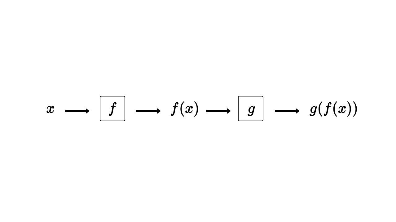
A diagram of connected input-output processes

First, let’s define these functions as the following.

$f(x) = x^{2}+5$

$g(x)=3x-4$

Next, we’ll evaluate $f(7)$ to produce the value $f(7) = (7)^{2} + 5 = 54$.

Finally, let’s take that $54$ and pass it as the input to $g$, producing $g(54) = 3(54) - 4 = 158$.

We mathematicians typically express compositions using the notation $g(f(x))$ or $(g \circ f)(x)$, both read “$g$ of $f$ of $x$”. In the previous example, we evaluated the composition $g(f(7))$ in two steps. You could also simplify the composition algebraically to start. The output of the function $f$ has become the input to the function $g$, so you can replace $g$’s argument $x$ with $f(x)$.

$f(x) = x^{2} + 5$

$g(x) = 3x - 4$

$g(f(x)) = 3 \cdot f(x) - 4$

Now, it’s easy to substitute $f(x)$ as follows.

$g(f(x)) = 3 (x^{2}+5) - 4$

$g(f(x)) = 3x^{2} + 15 - 4$

$g(f(x)) = 3x^{2} + 11$

Evaluating $g(f(x))$ is just a matter of substituting a number for $x$ into this final expression and computing the value.

$g(f(7)) = 3(7)^{2} + 11$

$g(f(7)) = 3(49) + 11$

$g(f(7)) = 158$

Composing functions in code maps neatly to the mathematical notation we just covered.

Example 3.5a Composing two functions

String Interlude

JavaScript’s data type for text is called a string. You can create strings by putting alphanumeric characters and even emoji between pairs of single '' or double "" quotes. Let’s display a string on the canvas by passing one as the first argument to p5’s text() function.

Example 3.5b Displaying strings

You could also combine, or concatenate, strings with other strings using the + operator.

Example 3.6a Concatenating strings with strings

Let’s end our brief introduction to strings by concatenating the left-hand side of our equation, a string, with the right-hand side, a floating point number.

Example 3.6b Concatenating strings with numbers

Now that we can visualize our algebraic work, let’s return to composition. Composition, as with any new mathematical technique, requires careful consideration to use correctly. Let’s compose the function $g(x) = 3x-4$ with the function $h(x) = \frac{1}{x}$.

$g(x) = 3x - 4$

$h(x) = \frac{1}{x}$

$h(g(x)) = \frac{1}{g(x)} = \frac{1}{3x - 4}$

Now, let’s try evaluating $h(g(\frac{4}{3}))$.

$h(g(\frac{4}{3})) = \frac{1}{3(\frac{4}{3}) - 4}$

$h(g(\frac{4}{3})) = \frac{1}{4 - 4}$

$h(g(\frac{4}{3})) = \frac{1}{0}$

Uh oh. Division by zero is undefined, so the denominator of $h(x)$ can’t be $0$. Since $g(\frac{4}{3}) = 0$, we need to restrict the domain of the composition $h(g(x))$ to all real numbers except $\frac{4}{3}$.

\[D : \{ n \: | \: n \in \mathbb{R} \: and \: n \ne \frac{4}{3} \}\]

Exercise 3.10 Compose the functions $a(x) = \sqrt{x} + 2$ and $b(x) = 7x + 11$ both ways. That is, find the algebraic expressions for $a(b(x))$ and $b(a(x))$ and note their domain and range. Does the order of composition matter? Explain why or why not in plain English.

Inverses Revisited

Let’s conclude this section by considering a special case of composition: a function and its inverse. I’ll define the function $q$ as $q(x) = 3x + 5$ and its inverse $q^{-1}(x) = \frac{x-5}{3}$. Frist, let’s evaluate the composition $q(q^{-1}(10))$ by starting with the inner function.

$q^{-1}(10) = \frac{10 - 5}{3} = \frac{5}{3}$

$q( \frac{5}{3}) = 3(\frac{5}{3}) + 5 = 5 + 5 = 10$

Interesting. Our input of $10$ produced an output of $10$. I wonder if that’s just a coincidence. Let’s try another input value, this time something negative.

$q^{-1}(-4) = \frac{-4 - 5}{3} = \frac{-9}{3} = -3$

$q(-3) = 3(-3) + 5 = -9 + 5 = -4$

OK, two for two. How about we see what happens when we compose these inverses algebraically?

$q(q^{-1}(x)) = 3 \cdot q^{-1}(x) + 5$

$q(q^{-1}(x)) = 3( \frac{x-5}{3}) + 5$

$q(q^{-1}(x)) = x - 5 + 5$

$q(q^{-1}(x)) = x$

How about that? Composing a function and its inverse results in… nothing happening at all. The output value is just the input! If you think about this result, it has some intuitive appeal. Inverting a function requires applying each operation in reverse. If you run a process forward, then immediately reverse each step, you wind up right where you started.

OK, I think you’re ready to apply composition as part of a quick financial analysis.

Exercise 3.11 Imagine opening a small business that specializes in data visualization. Let’s say you charge $\$ 30$ per hour to help local organizations to communicate their work by making interactive charts and simulations.

Write a short program that calculates how much tax you would owe at the end of a year based on the number of hours that you work. For simplicity, assume all of your income is taxed at $15 \%$.

Hint: write two functions and compose them.

Exercise 3.12 In this exercise, you will write another program that more accurately reflects income taxes in the United States. Use the marginal tax rates in Table 3.7 to compute the amount of income tax you owe. This system is a little complex, so let’s walk through a slightly simplified example together. If you worked $2,000$ hours and earned $\$ 60,000$, then your income would be taxed as follows.

$\$ 9,950$ at $10 \%$

$\$ 40,525 - \$ 9,951 = \$ 30,574$ at $12 \%$

$\$ 60,000 - \$ 40,526 = \$ 19,474$ at $22 \%$

All together, you would owe $\$ 9,950 \times 0.10 + \$ 30,574 \times 0.12 + \$ 19,474 \times 0.22 = \$ 8,948.16$. From a taxable income of $\$ 60,000$, your effective tax rate would be the following:

$\frac{ \$ 8,948.16 }{ \$ 60,000 } = 0.149 = 14.9 \%$

Hint: write two functions and use composition again, this time accounting for different tax brackets. If-statements and inequalities are your friends here.

Table 3.7 United States single filer tax rates for 2021 Courtesy irs.gov

Income	Rate
$\$ 0 – \$ 9,950$	$10 \%$
$\$ 9,951 – \$40,525$	$12 \%$
$\$40,526 – \$86,375$	$22 \%$
$\$86,376 – \$164,925$	$24 \%$
$\$164,926 – \$209,425$	$32 \%$
$\$209,426 – \$523,600$	$35 \%$
$\gt \$523,600$	$37 \%$

Reference

Precalculus / Chapters 1 and 2

This work is licensed under a Creative Commons Attribution-NonCommercial-ShareAlike 4.0 International License.

Income	Rate
\(\$ 0 – \$ 9,950\)	\(10 \%\)
\(\$ 9,951 – \$40,525\)	\(12 \%\)
\(\$40,526 – \$86,375\)	\(22 \%\)
\(\$86,376 – \$164,925\)	\(24 \%\)
\(\$164,926 – \$209,425\)	\(32 \%\)
\(\$209,426 – \$523,600\)	\(35 \%\)
\(\gt \$523,600\)	\(37 \%\)

\(x\)	-1	0	1	2
\(q(x)\)	3	5	7	9

\(x\)	-2	-1	0	1	2
\(q(x)\)	4	1	0	1	4

\(x\)	-2	-1	0	1	2
\(q(x)\)	ERROR	ERROR	0	1	4

\(x\)	-1	0	1	2
\(g(x)\)	3	5	7	9