Tutorial 2. Linear Systems
There’s definitely, definitely, definitely no logic
To human behaviour— “Human Behaviour” by Björk
I’m as excited as you are about making a meteor fly, so let’s take the complexity of our systems up a notch. We’ll set multiple objects in motion in this section and see what we can learn about their behavior.
2.1 Systems of Equations
Testing Solutions
In the last chapter, you applied linear equations as a mathematical model for the path of a meteor. As the meteor’s \(x\)-coordinate increased, its \(y\)-coordinate increased, and we related the two using an equation like the one below.
\(y = 0.5x + 50\)
If you substituted \(10\) for \(x\), you could evaluate the right-hand side to find, or solve for, \(y\).
\(y = 0.5 \cdot 10 + 50\)
\(y = 105\)
You could use the same approach to find every coordinate pair along the meteor’s path. Substituting the coordinate pair \((10,55)\) into the equation \(y=0.5x+50\) makes both sides equal, so we call it a solution to the equation.
How about the coordinate pair \((10,60)\)?
\(60=0.5 \cdot 10 + 50\)
\(60 \ne 55\)
No luck. The symbol \(\ne\) means “does not equal.” \((10,60)\) is not a solution to this equation.
OK, so we can map out all the points along an object’s path. But what if there were multiple objects moving along multiple paths?
Solving Equations
In the film Gravity, a Space Shuttle is destroyed by a barrage of space debris, forcing the survivors to find another way home to Earth before the debris completes another orbit and threatens them again. Let’s try to help out the astronauts by constructing a simulation of the Shuttle-debris system.
A Space Shuttle and debris in Earth’s orbit.
\(\mapsto\) Outer space is an empty, infinite, two-dimensional surface. The Space Shuttle is a point moving along the straight path described by the equation \(y=0.5x+50\). The debris is also a point moving along a straight path, this one described by the equation \(y= -0.5x+150\).
The coordinates of both objects are ordered pairs of floating point numbers. The Space Shuttle’s initial position is \((0,150)\). The debris’ initial position is \((0,50)\).
First, paint the sky. Next, select a pencil color & weight. Then, update the position of each object. Finally, draw a point at each object’s position.
Example 2.1 A collision
At the beginning of the film, Mission Control warns the astronauts that danger is coming. In real life, the United States Space Surveillance Network tracks objects in Earth’s orbit using a variety of sensing equipment. The team records the types of objects, when they were launched, their orbits, and their sizes. NASA uses this data to construct models that predict collisions like the one in Gravity.
While we don’t have a giant network of sensors and computers, we do have all the tools we need to figure out where the paths of our simulated Shuttle and debris cross. Let’s combine the equations describing each object’s path into a system of equations.
\(y = 0.5x + 50\)
\(y = -0.5x + 150\)
A system of equations is a set of related equations. There are infinitely many possible \((x,y)\) coordinate pairs, but only one solves both of these equations. For example, the point \((50,75)\) solves the equation for the Shuttle’s path.
\(75 = 0.5 \cdot 50 + 50\)
\(75 = 25 + 50\)
\(75 = 75\)
But does it also solve the equation for the debris’ path?
\(75 = -0.5 \cdot 50 + 150\)
\(150 = -25 + 150\)
\(150 \ne 125\)
No luck. We could try guessing and checking other coordinate pairs, but we might be at it for a while. There are many good techniques for solving systems of linear equations and we need a few additional ideas to apply them. Let’s start with a simpler case.
Math that uses letters as placeholders for numbers is known as algebra. Those placeholders, or variables, can show up anywhere we establish a relationship. Take the equation below as an example.
\(2 + 3 = 5\)
What if I wrote the following equation instead?
\(x + 3 = 5\)
We’ll use this example as a starting point for finding “unknown” values like \(x\), also called solving an equation. Given \(x+3 =5\), I want to come up with an algorithm that solves for \(x\). Let’s simplify again.
We know the following equation relates \(2\), \(3\), and \(5\).
\(2 + 3 = 5\)
Figure 2.1 Three hops to the right
You could express the same relationship another way by rearranging the equation a bit.
\(2 = 5 - 3\)
Figure 2.2 Three hops to the left
At this point you might think, “OK, the numbers \(2\) and \(5\) are \(3\) units apart. But what does that have to do with finding unknowns?” Everything, as it turns out.
We can think of the original equation \(2+3=5\) as running “forward” from the starting point \(2\). In this view, the second equation \(2=5-3\) runs “backward”. Running an operation backward is known as inverting the operation. And something interesting happens when we apply an operation and its inverse together.
\(2 + 3 - 3 = 2\)
Figure 2.3 Hopping back and forth
We’re right back where we started! Operations and their inverses undo each other; it’s like nothing happened at all. This fact is key to solving equations.
In math, the \(=\) symbol is an ironclad statement of equality. The left-hand side must equal the right-hand side, now and always. If you make a change to the left, you’d better do the same to the right. Let’s take the original equation one more time and invert the \(+3\) operation.
\(2 + 3 - 3 = 5 - 3\)
Or simplified:
\(2 = 2\)
Now, let’s apply identical reasoning to the equation with the variable \(x\).
\(x + 3 = 5\)
\(x + 3 - 3 = 5 - 3\)
\(x = 2\)
OK, let’s see that process one more time with a different example.
\(x - 2 = 10\)
\(x - 2 + 2 = 10 + 2\)
\(x = 12\)
Exercise 2.1 Given the equation \(x-5=10\), solve for \(x\). Then, describe the algorithm you used to solve for \(x\) in plain English.
Operator Precedence
Inverting addition and subtraction seems to work just fine, but what happens when you include other operations? Let’s take the path of our Shuttle.
\(y = 0.5x + 50\)
How would you determine the Shuttle’s \(x\)-coordinate when its \(y\)-coordinate is \(150\)?
\(150 = 0.5x + 50\)
It seems like we could invert this equation to solve for \(x\), but I’m not certain of how to proceed now that multiplication is in the mix. Figuring this out requires a brief interlude to discuss the order, or precedence, of mathematical operations.
If you come across an expression like \(2 \cdot 3 + 4\), the mathematical community has agreed that you should multiply before adding. You can compute the value produced in this example as follows.
\(2 \cdot 3 + 4\)
\(6 + 4\)
\(10\)
We’ve seen the computation run forward, so let’s go backward. The last operation applied was \(+4\), so let’s invert that first.
\(10 = 2 \cdot 3 + 4\)
\(10 - 4 = 2 \cdot 3 + 4 - 4\)
\(6 = 2 \cdot 3\)
You can view the multiplication as \(2\) multiplying \(3\) or as \(3\) multiplying \(2\). I’ll go with the former and undo multiplication by \(2\).
\(\frac{6}{2} = \frac{2 \cdot 3}{2}\)
\(3 = 3\)
How about we substitute one of the operands for a variable and solve for it?
\(10 = 2x + 4\)
\(10 - 4 = 2x + 4 - 4\)
\(6 = 2x\)
\(\frac{6}{2} = \frac{2x}{2}\)
\(3 = x\)
It’s been quite a journey, but I think we’re ready to plot a course for our Shuttle.
\(150 = 0.5x + 50\)
\(150 - 50 = 0.5x + 50 - 50\)
\(100 = 0.5x\)
\(\frac{100}{0.5} = \frac{0.5x}{0.5}\)
\(200 = x\)
Exercise 2.2 Find the \(x\)-coordinate of the Shuttle when its \(y\)-coordinate is \(180\). Then, describe the algorithm you used to solve for \(x\) in plain English.
The order of mathematical operations is bundled up nice and neat in the acronym PEMDAS.
Parentheses
Exponents
Multiplication
Division
Addition
Subtraction
Let’s focus on MDAS for now as they are key to linear relationships. Multiplication and division have the same precedence. Consider the example below.
\(3 \cdot 10 \div 5\)
You could compute \(3 \cdot 10 = 30\), then divide \(30 \div 5\) to produce \(6\). Or you could start by dividing \(10 \div 5 = 2\) before multiplying \(3 \cdot 2\) to produce \(6\). There are multiple pathways to the correct answer!
There is a similar story for addition and subtraction.
\(3 + 10 - 5\)
You could compute \(3 + 10 = 13\), then subtract \(13 - 5\) to produce \(8\). Or you could start by subtracting \(10 - 5 = 5\) and add \(3 + 5 = 8\). Once again, multiple pathways!
Exercise 2.3 Evaluate the expression \(10 \cdot 5 \div 2 + 5\).
Exercise 2.4 Evaluate the expression \(10 ÷ 5 - 2 \cdot 5\).
Solving Systems
We’re on a tight schedule to be of any help to NASA. Let’s figure out the coordinates \((x,y)\) where the paths of the Shuttle and debris intersect. Recall the system of equations describing the scenario.
\(y = 0.5x + 50\)
\(y = -0.5x + 150\)
There are infinitely many points along each object’s path, and the variables \(x\) and \(y\) are placeholders for all of them. The Shuttle and debris were moving before they collided, and they continued moving afterward. Those variables \(x\) and \(y\) that solved one equation at a time must now solve both equations simultaneously.
Substitution
Algebraic techniques help us solve systems of equations because we really do mean that the \(y\) in the first equation is the very same \(y\) in the second equation. Consider the following simplified case for a moment.
\(a = 5\)
\(b = 5\)
\(a = b\)
The same transitive property of equality applies to systems of equations.
\(y = 0.5x + 50\)
\(y = -0.5x + 150\)
\(0.5x + 50 = -0.5x + 150\)
Now we have one equation with one unknown. Let’s solve it for \(x\)!
\(0.5x + 50 = -0.5x + 150\)
\(0.5x + 0.5x + 50 = -0.5x + 0.5x + 150\)
\(x + 50 = 150\)
\(x + 50 - 50 = 150 - 50\)
\(x = 100\)
And now that we’ve found \(x\), we can substitute the value back into one of the original equations to find \(y\).
\(y = 0.5 \cdot 100 + 50\)
\(y = 50 + 50\)
\(y = 100\)
We also could have gone with the other equation.
\(y = -0.5 \cdot 100 + 150\)
\(y = -50 + 150\)
\(y = 100\)
Example 2.2 Predicting collision
As you may expect, there’s more than one way to solve this problem. Let’s examine a different algorithm that combines equations to find solutions.
Elimination and Back Substitution
First, I’m going to determine the value of \(y\) by eliminating the variable \(x\) from an equation. Unlike the substitution algorithm, which rewrote one variable in terms of another, I’ll eliminate \(x\) by adding the top equation to the bottom equation. As usual, let’s motivate this idea by considering a simpler case. Take the equations below.
\(20 = 4 \cdot 5\)
\(2x = x + x\)
I could add the two left-hand sides to produce \(2x + 20\). On the right-hand side, I would have \(x + x + 4 \cdot 5\). But do these combined expressions equal each other? We’ll follow this one step-by-step.
\(2x + 20 = x + x + 4 \cdot 5\)
\(2x + 20 = x + x + 20\)
\(2x + 20 = 2x + 20\)
Those \(=\) symbols mean that the expressions on the left- and right-hand sides are equal. When we add the same thing to each side of an equation, we maintain equality. You may hear this called the additive property of equality when you’re out at parties. Now, let’s use this property to eliminate the variable \(x\) and solve for \(y\).
\(y = 0.5x + 50\)
\(y = -0.5x + 150\)
\(y + y = -0.5x + 0.5x + 150 + 50\)
\(2y = 200\)
\(\frac{2y}{2} = \frac{200}{2}\)
\(y = 100\)
The \(y\)-value we just found resulted from combining information stored in separate equations. This is the \(y\)-value both equations share. But what about \(x\)? Well, we know that \(y = 100\), so let’s substitute that part of our solution back into the system.
\(100 = 0.5x + 50\)
\(100 - 50 = 0.5x + 50 - 50\)
\(50 = 0.5x\)
\(\frac{50}{0.5} = \frac{0.5x}{0.5}\)
\(100 = x\)
You’ve now seen two of many possible algorithms for solving systems of linear equations. Practice with them a bit before we build up the logical foundations you need to explore systems of linear inequalities.
Exercise 2.5 Solve the system of equations below using Substitution. Then, solve it using Elimination and Back Substitution. Describe how each algorithm works in plain English.
\(y = 0.25x + 100\)
\(y = -0.75x + 300\)
2.2 Logic
In the novel 1984, the main character is brainwashed into accepting that \(2 + 2 = 5\) is true. The scene depicts the ultimate flex of power by an oppressive government. Let’s lay some logical foundations to ensure we always maintain our grasp on the truth.
Boolean Algebra
You just tested a few different coordinate pairs \((x,y)\) to determine whether or not they solved an equation. The test could only have gone one of two ways: success or failure, yes or no, true or false. There is an entire branch of algebra called Boolean algebra dedicated to studying these two truth values, which we usually write as \(1\) (true) and \(0\) (false). There are not infinitely many truth values like there are numbers; there are only \(1\) and \(0\).
A truth value can correspond to a situation in the real world. For example, I could claim, “The sun is up”. This claim happens to be false in my neck of the woods as I write this sentence. I can express this idea using the variable \(s\) to represent sunniness.
\(s = 0\)
Even though the sun has already set on this particular day, the sky above me is still momentarily deep blue. I can claim “The sky is blue” and express this blueness, \(b\), matter-of-factly.
\(b = 1\)
OK, we have variables with assigned values. But what can we actually do with them?
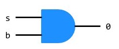
Let’s begin by combining \(s\) and \(b\) using our first logical operation: conjunction, also known as AND. The expression \(s \land b\) means “\(s\) is true AND \(b\) is true”. The sky above my front porch is blue, but the sun is not up, so the combined statement is false. We could write this concisely as \(s \land b = 0\).
There is a special set of diagrams called logic gates that depict the results of applying logical operations. Each logic gate has a distinctive shape. Below is the diagram for the AND logic gate.
Figure 2.4 The AND logic gate
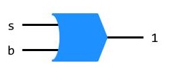
One of the variables \(s\) and \(b\) is true, and we can test for such a condition using the disjunction operation, also known as OR. A disjunction is true if at least one of its operands is true. I could claim “The sun is up OR the sky is blue” and that would be true because \(b = 1\). We could express idea this as \(s \lor b = 1\).
Like AND, OR also has its own logic gate.
Figure 2.5 The OR logic gate
The following truth table organizes all of the facts we’ve established about the view of the sky from my front porch.
Table 2.1 A truth table’s view of my piece of sky
| \(s\) | \(b\) | \(s \land b\) | \(s \lor b\) |
|---|---|---|---|
| \(0\) | \(1\) | \(0\) | \(1\) |
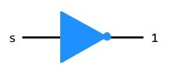
The final logical operation we’ll discuss is negation, also known as NOT. The NOT operation simply flips a truth value from \(1\) to \(0\) or from \(0\) to \(1\). Let’s take the variable \(s\) and negate it using the NOT operator, \(\lnot\).
\(s = 0\)
\(\lnot s = 1\)
NOT is a unary operation, meaning we only apply it to a single truth value at a time. AND and OR are both binary operations, meaning we have to provide a pair of operands.
Not to be left out, NOT also has its own logic gate.
Figure 2.6 The NOT logic gate
And that’s all you need to get started with logic! You can compose logical operations just like you do arithmetic operations. For example, let’s figure out how to cross the street safely using logic. I’ll define the variables \(l\) and \(r\) to represent vehicle traffic from the left and traffic from the right, respectively.
If you were trying to cross a busy street, you would want to avoid vehicles. In logical terms, you would check to see that both \(l = 0\) and \(r = 0\). “No vehicles on the left? No vehicles on the right? OK, let’s go!” This condition is easily expressed by combining operations \(\lnot l \land \lnot r = 1\).
Exercise 2.6 Complete the following truth table for two boolean variables \(x\) and \(y\).
| \(x\) | \(y\) | \(x \land y\) | \(x \lor y\) |
|---|---|---|---|
| \(0\) | \(0\) | ||
| \(0\) | \(1\) | ||
| \(1\) | \(0\) | ||
| \(1\) | \(1\) |
Exercise 2.7 Compute the value of the expression \(\lnot (1 \land 1)\).
Exercise 2.8 Compute the value of the expression \((1 \land 0) \lor (1 \lor 0)\).
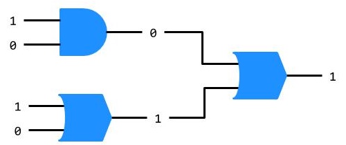
Exercise 2.9 Rewrite the following logic circuit as an equivalent logical expression.
Exercise 2.10 Complete the following truth table for two boolean variables \(x\) and \(y\). What do you notice?
| \(x\) | \(y\) | \(\lnot (x \land y)\) | \(\lnot x \lor \lnot y\) | \(\lnot (x \lor y)\) | \(\lnot x \land \lnot y\) |
|---|---|---|---|---|---|
| \(0\) | \(0\) | ||||
| \(0\) | \(1\) | ||||
| \(1\) | \(0\) | ||||
| \(1\) | \(1\) |
Branching
Logic is a big deal for computation, from the way the machines are physically built to the way we program them. Conditional statements let us test conditions and make decisions while a program executes. For example, let’s revisit the collision scene from Gravity.
Example 2.3 Collision revisited
The simulation works fine, but it doesn’t really convey the full drama of the situation. Let’s revise our system a bit to account for the additional debris generated upon collision.
A Space Shuttle and debris in Earth’s orbit.
\(\mapsto\) Outer space is an empty, infinite, two-dimensional surface. The Space Shuttle is a point moving along the straight path described by the equation \(y = 0.5x + 50\). The debris is also a point moving along a straight path, this one described by the equation \(y = -0.5x + 150\). After colliding, each object leaves a trail of smaller debris along its path.
The coordinates of both objects are ordered pairs of floating point numbers. The Space Shuttle’s initial position is \((0,50)\). The debris’ initial position is \((0,150)\).
First, test for collision and set the alpha value for the sky. Then, paint the sky. Next, update the position of each object. After that, select a pencil color & weight. Finally, draw a point at each object’s position.
Lucky for us, you already solved this system and know that the two objects collide at \((100,100)\). As the sketch continues running, the Shuttle and debris continue moving to the right. We can test for this using an if statement.
if (condition) {
  // things to do if condition is true
}
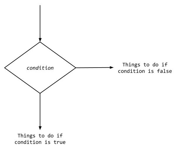
If statements present a logical crossroads in a program. The first line of the if statement is called a header. The header begins with if, defines the condition to test in between a pair of parentheses (), then opens a pair of {}. If the condition is true, JavaScript will execute the set of statements between the {}, also known as the if statement’s body.
if (condition) {
  thingOne() // this is part of the body
  thingTwo() // this too!
}

thingThree() // this is not
In the Gravity example, we’re testing whether or not the value of the variable x is greater than 100. JavaScript has the following relational operators that work as you would expect for numbers.
Table 2.2 JavaScript’s relational operators
| \(Math\) | Code |
English |
|---|---|---|
| \(=\) | === |
Equal to |
| \(\ne\) | !== |
Not equal to |
| \(>\) | > |
Greater than |
| \(<\) | < |
Less than |
| \(\ge\) | >= |
Greater than or equal to |
| \(\le\) | <= |
Less than or equal to |
Applying a relational operator produces a boolean value. For example, the expression 2 + 2 === 5 produces the boolean value false because, well, math. 2 + 2 === 4, on the other hand, produces the value true. These sorts of logical expressions are called boolean expressions.
if (x > 100) {
  // things to do if x > 100
}
Example 2.4 A more impactful collision
Exercise 2.11
Duplicate your original collision sketch and add a few effects. How should the visual appearance of the Shuttle and debris change after impact?
You can also test multiple conditions together. Thinking back to the meteor sketch, how about we make the meteor glow red as it passes over the middle half of the canvas? In other words, when \(x \ge 50\) AND \(x \le 150\).
if (x >= 50 && x <= 150) {
  stroke('tomato')
}
&& is one of JavaScript’s boolean operators along with || and !. These JavaScript operators function identically to the logical operators you just studied.
Recall our earlier \(2 + 2\) example from the novel 1984. Notice you can test for the same condition using different boolean operators.
if (2 + 2 !== 4) {
  resist()
}
or
if (!(2 + 2 === 4)) {
  resist()
}
Example 2.5 A colorful meteor
Reading through this code, it isn’t immediately clear that ghostwhite is meant to be the default stroke color. You could make this more explicit by adding an else clause to your conditional statement. Here is an example of the syntax.
if (condition) {
  // things to do if condition is true
} else {
  // things to do if condition is false
}
The conditional statement now has two distinct pathways, or branches, that may be followed depending on the truth value of the condition.
Figure 2.7 Flow of execution with two branches
You could reorganize your sketch to reflect this structure like so.
At this point, you might say, “Branches seem useful, but what if I want more than two in my program?” Say no more! You can chain conditionals together using an else if statement (a combination of “else” and “if”). In a chained conditional, conditions are tested in the order they are written, and only the first branch whose condition is true will execute.
if (condition1) {
  thingOne()
} else if (condition2) {
  thingTwo()
} else {
  thingThree()
}
Example 2.6 A multicolor meteor
Exercise 2.12 Change the previous example so that the following conditions are tested in this order. Can you explain what happened?
if (x >= 50) {
  stroke('tomato')
} else if (x >= 150) {
  stroke('crimson')
} else {
  stroke('ghostwhite')
}
Exercise 2.13 Duplicate one of your previous sketches and modify its behavior using conditional statements. Use at least one other relational and one other boolean operator.
2.3 Iteration
The logical building blocks you assembled in the last two sections let you create branches and make decisions in your programs. In this section, we’ll use many of the same building blocks to form another type of control flow: repetition.
while statements
In Exercise 1.18, you drew a constellation by calling the point() function repeatedly with different arguments. Let’s revisit this exercise using the constellation Orion as a starting point. We’ll focus on Orion’s Belt, which consists of the stars Alnitak, Alnilam, and Mintaka.
Orion’s Belt
\(\mapsto\) Outer space is an empty, infinite, two-dimensional surface. Stars are points of light within this plane.
Star coordinates are ordered pairs of floating point numbers.
Table 2.3 The “Orion’s Belt” data set
| Star Name | \(x\) | \(y\) |
|---|---|---|
| Alnitak | 25 | 100 |
| Alnilam | 100 | 100 |
| Mintaka | 175 | 100 |
First, paint the night sky. Then, select a pencil color & weight. Finally, draw a point at each star’s position.
Example 2.7 Orion’s Belt
The stars Alnitak and Mintaka are actually star systems; each system is made up of multiple stars orbiting one another. I’ll use this fact as my creative license to adjust Orion’s Belt a little. For starters, how about we draw Orion’s Belt with all of the major stars in each system? Let’s keep things simple by assuming all of the stars are the same size and are aligned horizontally in the sky.
Table 2.4 Expanded “Orion’s Belt” data set
| Star Name | \(x\) | \(y\) |
|---|---|---|
| Alnitak Aa | 25 | 100 |
| Alnitak Ab | 50 | 100 |
| Alnitak B | 75 | 100 |
| Alnilam | 100 | 100 |
| δ Ori Aa1 | 125 | 100 |
| δ Ori Aa2 | 150 | 100 |
| δ Ori Ab | 175 | 100 |
Example 2.8 Adjusting Orion’s Belt
The visual result looks good, but the code worries me a little. Notice that I wrote seven nearly identical copies of the same statement to draw the stars. This approach works fine to get started but imagine writing a program that needs to repeat an instruction dozens of times. Or millions of times. Writing each variant by hand would be tedious and error prone. JavaScript’s while statement makes repetition, or iteration, simple.
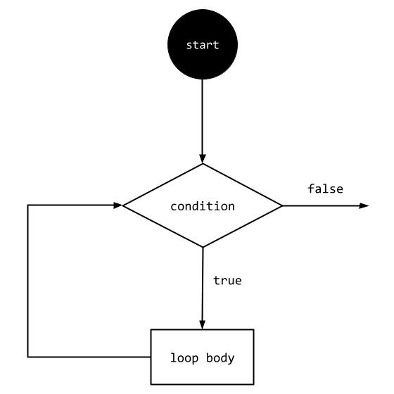
while (condition) {
  // this is the loop body
  // statements in here repeat while condition is true
  thingOne()
  thingTwo()
}
while statements are structured similarly to if statements; they have a header with a condition and a body with code that might be executed. Each statement in the body executes in order, from top to bottom, repeatedly, until the condition in the header is false. Iterative control structures like this are commonly known as loops.
Figure 2.8 Flow of execution in a while loop
Let’s use a while loop to simplify our sketch of Orion’s Belt. Reviewing the previous example, the only difference between the stars is their \(x\)-coordinates. We know where our \(x\)-coordinates start, where they stop, and how much space is between them. This is all the information we need to simplify our work by using a loop.
Example 2.9 Orion’s Belt with iteration
Not too shabby! Given an initial value for x, the while statement draws a point, then increments x by 25, and repeats this process until x is greater than 175.
We could change one line of code from the previous example to pack twice as many stars in the same region of sky.
Example 2.10 Bedazzling Orion’s Belt
Exercise 2.14
Modify the sketch above to draw a row of stars in a different arrangement. What is the initial value of your loop variable x? What condition do you test to end the loop’s execution? How much do you increment x by during each iteration?
You might say, “OK, but what if I turned my head a little? Could I draw the stars along a vertical line instead?” Sure! In this case, you could keep the value of x constant while varying y.
Example 2.11 Switching axes from \(x\) to \(y\)
Infinite Loops
while statements are powerful tools that should be used with care. Consider the example below.
while (true) {
  thingOne()
  thingTwo()
}
true is a keyword in JavaScript that corresponds to a boolean value of, you guessed it, true. If a while statement’s condition is always true, then it will continue looping forever, thus creating an infinite loop. Unintended infinite loops are bad news. Let’s examine a slightly modified version of the loop from the previous sketch.
let y = 25
while (y <= 175) {
  point(100, y)
}

y += 25 // oops
Notice that I incremented y outside of the loop body. This means that y isn’t incremented after each iteration. Instead, the value of y will always be 25, which is always less than or equal to 175, so the condition 25 <= 175 is always true. The loop never stops executing! If you ran this code, your web browser might give you a friendly notification to stop the sketch before it grinds your computer to a halt.
Exercise 2.15 The code snippet below is meant to draw a horizontal row of points across the canvas. Instead, it creates an infinite loop. Identify the error and fix it. Explain the problem and your solution in plain English.
let x = 0
let y = 100
while (x < 200) {
  point(x, y)
  x += 10
}
Exercise 2.16
Create a sketch that uses a while statement to draw points along a diagonal line. Review the code snippet below as a hint.
let x = 0
while (x < 200) {
  // >> compute y here
  point(x, y)
  x += 10
}
Exercise 2.17
In the last tutorial, we defined an algorithm for multiplying two integers \(a \cdot b\) as repeated addition \(b + b + ... + b\). Fill in the missing code below to express the same algorithm in JavaScript using a while loop.
let a = 5
let b = 3
let product = 0
let i = 0
while (i < a) {
  // >> compute product here
  i += 1
}
Exercise 2.18
Review the algorithms for integer division and exponentiation, then implement them in JavaScript using a while loop. The subtraction assignment -= and multiplication assignment *= operators might be helpful.
2.4 Systems of Inequalities
We began this chapter by analyzing a single linear equation in slope-intercept form: \(y = mx + b\). You could substitute any real number for \(x\) and compute the corresponding value of \(y\), making the ordered pair \((x,y)\) a solution to the equation. Let’s review a concrete example.
Given the following linear equation
\(y = 0.5x + 100\)
compute the value of \(y\) when \(x = 50\).
\(y = 0.5 \cdot 50 + 100\)
\(y = 25 + 100\)
\(y = 125\)
One solution to this equation is located at \((50,125)\). What if we tried \((50,126)\) instead?
\(126 = 0.5 \cdot 50 + 100\)
\(126 = 25 + 100\)
\(126 \ne 125\)
It turns out \((50,126)\) is not a solution to this particular equation, but there are infinitely many other solutions. For example, we could find solutions to the left and right of \((50,125)\) at \(x = 49\) and \(x = 51\).
\(y = 0.5 \cdot 49 + 100\)
\(y = 24.5 + 100\)
\(y = 124.5\)
\(y = 0.5 \cdot 51 + 50\)
\(y = 25.5 + 100\)
\(y = 125.5\)
You could use a while loop to quickly compute and visualize all of the solutions in the interval \(0 \le x \le 200\).
Example 2.12 Visualizing solutions to a linear equation
Mathematicians often express a change in the value of a variable with the Greek letter \(\Delta\), pronounced “delta”. Using this notation, we can express a change in the variable \(x\) as \(\Delta x\). I declare the variable dx on line 11 and use it to increment x on line 15 as a nod to our standard mathematical notation.
Testing Solutions
OK, the solutions to a linear equation generate a line. I wonder what shapes other linear relationships make. Let’s take the previous example and swap out the \(=\) symbol for a \(>\).
\(y > 0.5x + 100\)
You can test solutions to this linear inequality just as you did with linear equations. For example, let’s see if the coordinate pair \((50,125)\) produces a truth value of \(1\) when we substitute the values into our inequality.
\(125 > 0.5 \cdot 50 + 100\)
\(125 > 25 + 100\)
\(125 > 125\)
Uh oh. We evaluated the right-hand side of the inequality and produced a value of \(125\). But that resulted in a false statement; \(125\) is not greater than itself. We can conclude that \((50,125)\) isn’t a solution to this inequality. How about we move along the \(y-axis\) a little to \((50,126)\)?
\(126 > 0.5 \cdot 50 + 100\)
\(126 > 25 + 100\)
\(126 > 125\)
Success! Let’s go a little further along the \(y\)-axis to \((50,127)\).
\(127 > 0.5 \cdot 50 + 100\)
\(127 > 25 + 100\)
\(127 > 125\)
Interesting. Let’s try one more coordinate pair \((50,128)\) to see if this pattern holds.
\(128 > 0.5 \cdot 50 + 100\)
\(128 > 25 + 100\)
\(128 > 125\)
When \(x = 50\), we can pair it with any \(y > 125\) to solve the inequality \(y > 0.5x + 100\). You could automate this sort of test with a while loop.
Example 2.13 Testing solutions to a linear inequality
The sketch above fixes the value of x at 50 and tests solutions to the inequality for all y values in the interval \(0 \le y < 200\). Solutions along this column are colored black while other points are colored ghostwhite.
This is the first example we’ve seen of a while loop that includes an if statement in its body. You can put (almost) whatever code you want in the body of a while loop: function calls, arithmetic operations, if statements, and even other while loops. This last option opens up many interesting possibilities.
Nested Loops
You just tested hundreds of possible solutions to the inequality \(y > 0.5x + 100\) when \(x\) was fixed at \(50\). Let’s fully automate the process of testing solutions by iterating over the canvas’ \(x\)-axis just like we’re doing with its \(y\)-axis.
A quick note about the algorithm we are about to run: it is very inefficient and would normally grind your computer to a halt. By default, p5 executes each statement you place in the body of the draw() function in order, from top to bottom, repeatedly, about \(60\) times per second. Behind the scenes, you can imagine that the code you write in draw() is executing in the body of a while statement.
setup()  // all of your code bundled up

while (true) {
  draw() // all of your code bundled up
}
Testing individual solutions to a linear inequality requires computing once on each \((x,y)\) coordinate pair before drawing a point on the canvas–that’s roughly \(200 \cdot 200 = 40000\) operations! The algorithm is slow and produces the same results every time, so there is no need to repeat it.
In the next example and those that follow, I will call the noLoop() function once in setup() like so.
function setup() {
  createCanvas(400, 400)
  noLoop()
}
By calling noLoop(), you change p5’s behavior so that draw() only executes a single time. You can imagine p5 running the following code instead.
setup() // all of your code bundled up

draw()  // all of your code bundled up
Now, we can compute once on each \((x,y)\) coordinate pair, draw the corresponding point, and produce a single image. This adjustment should keep your computer happy, but it may still take a moment for the result to appear.
Example 2.14 Visualizing a linear inequality
The control structure you just created is called a nested loop. The outer loop increments the variable x while the inner loop increments the variable y and tests for solutions along each column of your canvas. And the result of all that computation? It turns out the set of \((x,y)\) coordinate pairs that solve our inequality, known as the solution set, forms a triangle-shaped region with the edges of the canvas. Neat! Can we make a rectangle?
Example 2.15 The rectangle inequality
Exercise 2.19 Modify the previous example to draw a new five-sided shape with your solution set. Closed shapes made by connecting three or more straight lines are known as polygons, and a five-sided polygon is known as a pentagon.
Exercise 2.20 Ellsworth Kelly’s “Austin” is a serene little chapel located on the campus of the University of Texas at Austin. Its walls feature a series of fourteen black and white marble panels that look suspiciously like linear inequalities. Use Kelly’s panels as inspiration for your own series of abstract images. How many images will you include in your series? What colors will you use? What shapes will you create?
Drawing with linear inequalities opens up a dizzying number of creative possibilities. But what if you just wanted to draw a rectangle in the middle of your canvas? Meeting this challenge requires expanding our modeling toolkit yet again.
Solving Systems
When you solved your first system of linear equations, you found the point \((x,y)\) where two lines intersected. In other words, you found the only ordered pair \((x,y)\) that solved both equations simultaneously. We’ll follow a very similar train of thought to solve systems of linear inequalities.
For starters, let’s try consider the system \(y < x + 150\) and \(y > 75\). We can test possible solutions \((x,y)\) against both inequalities using the && operator.
Example 2.16 A system of linear inequalities
OK, but how would we draw that rectangle in the middle of the canvas? You can think of a rectangle as the set of points between a pair of \(x\)-values and a pair of \(y\)-values. For example, we could take all of the points where \(x > 75\) AND \(x < 125\) AND \(y > 100\) AND \(y < 160\).
Example 2.17 A more constrained system
At this point you might say, “This is great! But how do I draw multiple shapes?” Simple: define multiple systems of inequalities. I’d like to frame this part of the discussion by studying the work of another abstract painter, Piet Mondrian.
Figure 2.9 “Composition II in Red, Blue, and Yellow” Courtesy Wikimedia Foundation
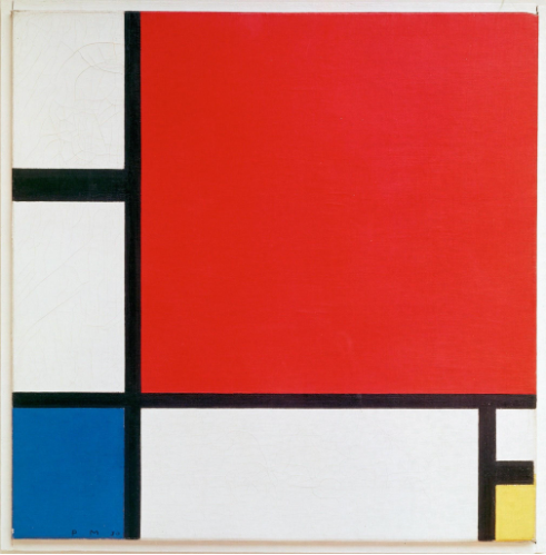
The painting “Composition II”
\(\mapsto\) Each colored region is the solution set to a system of linear inequalities.
The boundaries for each system of inequalities are either vertical or horizontal lines.
Table 2.5 The “Composition II” data set
| Name | Left \(x\) | Right \(x\) | Bottom \(y\) | Top \(y\) |
|---|---|---|---|---|
| Blue corner | 0 | 35 | 155 | 200 |
| Yellow corner | 188 | 200 | 183 | 200 |
| Red corner | 40 | 200 | 0 | 150 |
| Stripe 1 | 35 | 40 | 0 | 200 |
| Stripe 2 | 0 | 35 | 60 | 72 |
| Stripe 3 | 0 | 200 | 150 | 155 |
| Stripe 4 | 183 | 188 | 155 | 200 |
| Stripe 5 | 188 | 200 | 173 | 183 |
First, prime the canvas by painting it ghostwhite. Next, select the paint color by testing whether a point solves a system of inequalities. Finally, paint the point. Repeat for every point on the canvas.
Example 2.18 “Composition II”
Exercise 2.21 Spend a few minutes exploring WikiArt and find an abstract painting or painter who inspires you. Hilma af Klint and Mark Rothko are personal favorites of mine. Then, create a new sketch that uses systems of inequalities to draw your own abstraction. Is your sketch completely abstract or is it based on an object, place, emotion, etc.? What do you like most about your sketch? What was challenging about creating it?
Exercise 2.22 Visualize integer multiplication by building on your solution to Exercise 2.17. Use the starter code below to snap (very tiny) blocks together.
The noStroke() function removes edges p5 draws around text; doing so can make it easier to read some fonts. The fill() function sets the interior color of text. Note that the text() function takes three arguments: the text to be displayed, and the \(x\)- and \(y\)-coordinates where the text should appear.
The control structures you just studied make it possible to construct many useful computations. In the next chapter, we’ll raise the level of abstraction by bundling computations into functions you define. We’ll also have fun drawing with the many built-in shapes that p5 provides.
Reference
- Intermediate Algebra 2e / Chapter 3
- Precalculus / Chapter 9
This work is licensed under a Creative Commons Attribution-NonCommercial-ShareAlike 4.0 International License.